Optimal Transport in 2D

Let’s use the gradient of the Sinkhorn divergence to compute an Optimal Transport map.

Setup

import numpy as np
import matplotlib.pyplot as plt
import time

import torch
from geomloss import SamplesLoss

use_cuda = torch.cuda.is_available()
dtype = torch.cuda.FloatTensor if use_cuda else torch.FloatTensor

Display routines

from random import choices
from imageio import imread


def load_image(fname):
    img = imread(fname, as_gray=True)  # Grayscale
    img = (img[::-1, :]) / 255.0
    return 1 - img


def draw_samples(fname, n, dtype=torch.FloatTensor):
    A = load_image(fname)
    xg, yg = np.meshgrid(
        np.linspace(0, 1, A.shape[0]),
        np.linspace(0, 1, A.shape[1]),
        indexing="xy",
    )

    grid = list(zip(xg.ravel(), yg.ravel()))
    dens = A.ravel() / A.sum()
    dots = np.array(choices(grid, dens, k=n))
    dots += (0.5 / A.shape[0]) * np.random.standard_normal(dots.shape)

    return torch.from_numpy(dots).type(dtype)


def display_samples(ax, x, color):
    x_ = x.detach().cpu().numpy()
    ax.scatter(x_[:, 0], x_[:, 1], 25 * 500 / len(x_), color, edgecolors="none")

Dataset

Our source and target samples are drawn from measures whose densities are stored in simple PNG files. They allow us to define a pair of discrete probability measures:

\[\alpha ~=~ \frac{1}{N}\sum_{i=1}^N \delta_{x_i}, ~~~ \beta ~=~ \frac{1}{M}\sum_{j=1}^M \delta_{y_j}.\]

N, M = (100, 100) if not use_cuda else (10000, 10000)

X_i = draw_samples("data/density_a.png", N, dtype)
Y_j = draw_samples("data/density_b.png", M, dtype)

/home/code/geomloss/geomloss/examples/optimal_transport/plot_optimal_transport_2D.py:33: DeprecationWarning: Starting with ImageIO v3 the behavior of this function will switch to that of iio.v3.imread. To keep the current behavior (and make this warning disappear) use `import imageio.v2 as imageio` or call `imageio.v2.imread` directly.
  img = imread(fname, as_gray=True)  # Grayscale

Lagrangian gradient descent

def gradient_descent(loss, lr=1):
    """Flows along the gradient of the loss function.

    Parameters:
        loss ((x_i,y_j) -> torch float number):
            Real-valued loss function.
        lr (float, default = 1):
            Learning rate, i.e. time step.
    """

    # Parameters for the gradient descent
    Nsteps = 11
    display_its = [0, 1, 2, 10]

    # Use colors to identify the particles
    colors = (10 * X_i[:, 0]).cos() * (10 * X_i[:, 1]).cos()
    colors = colors.detach().cpu().numpy()

    # Make sure that we won't modify the reference samples
    x_i, y_j = X_i.clone(), Y_j.clone()

    # We're going to perform gradient descent on Loss(α, β)
    # wrt. the positions x_i of the diracs masses that make up α:
    x_i.requires_grad = True

    t_0 = time.time()
    plt.figure(figsize=(12, 12))
    k = 1
    for i in range(Nsteps):  # Euler scheme ===============
        # Compute cost and gradient
        L_αβ = loss(x_i, y_j)
        [g] = torch.autograd.grad(L_αβ, [x_i])

        if i in display_its:  # display
            ax = plt.subplot(2, 2, k)
            k = k + 1
            plt.set_cmap("hsv")
            plt.scatter(
                [10], [10]
            )  # shameless hack to prevent a slight change of axis...

            display_samples(ax, y_j, [(0.55, 0.55, 0.95)])
            display_samples(ax, x_i, colors)

            ax.set_title("it = {}".format(i))

            plt.axis([0, 1, 0, 1])
            plt.gca().set_aspect("equal", adjustable="box")
            plt.xticks([], [])
            plt.yticks([], [])
            plt.tight_layout()

        # in-place modification of the tensor's values
        x_i.data -= lr * len(x_i) * g
    plt.title(
        "it = {}, elapsed time: {:.2f}s/it".format(i, (time.time() - t_0) / Nsteps)
    )

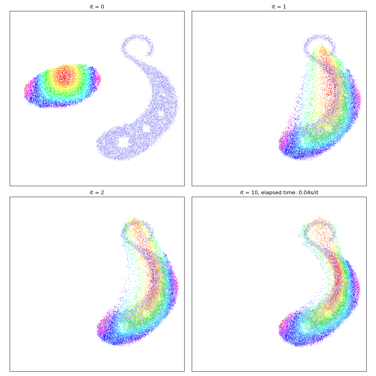
Wasserstein-2 Optimal Transport

Sinkhorn divergences rely on blurry transport plans \(\pi_{\varepsilon,\rho}^{\alpha,\beta}\), \(\pi_{\varepsilon,\rho}^{\alpha,\alpha}\) and \(\pi_{\varepsilon,\rho}^{\beta,\beta}\), solutions of the entropized transport problems that cannot be readily interpreted as deterministic maps.

However, when p = 2, we can interpret the gradient field \(v_i \,=\, \tfrac{1}{\alpha_i} \nabla_{x_i} \text{S}_{\varepsilon,\rho}(\alpha,\beta)\) as a Brenier-like transport plan, which maps source points \(x_i\) to a barycenter \(x_i+v_i\) of targets at scale \(\text{blur}\,=\,\sqrt{\varepsilon}\).

gradient_descent(SamplesLoss("sinkhorn", p=2, blur=0.1))

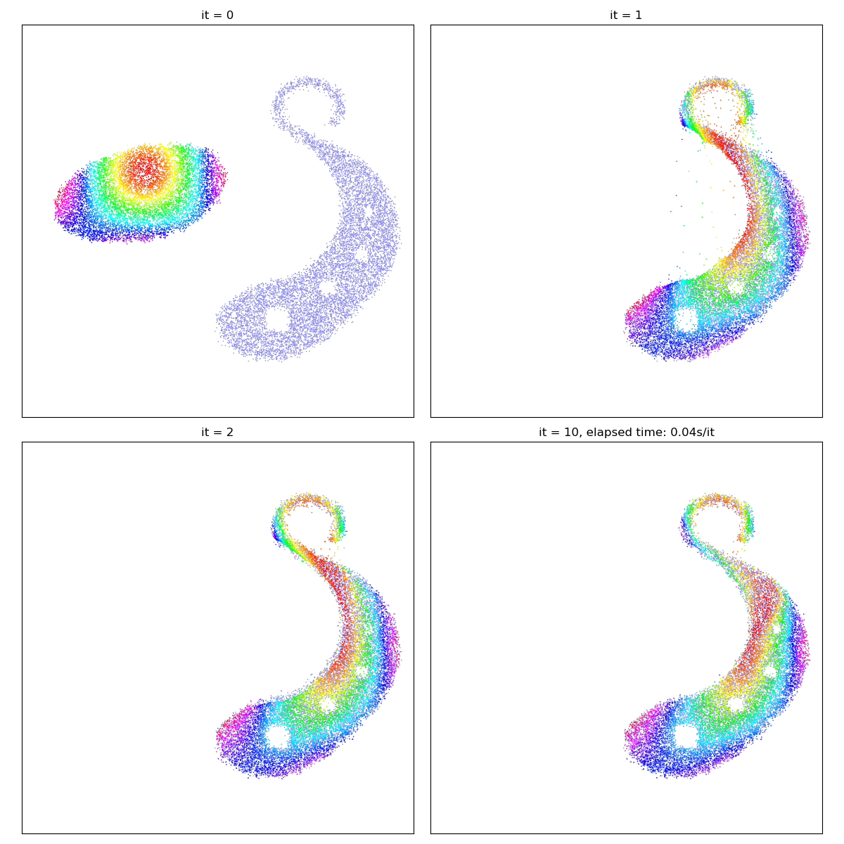
Crucially, as the blurring scale \(\sqrt{\varepsilon}\) tends to zero, \(\pi_{\varepsilon,\rho}^{\alpha,\beta}\) converges towards a “genuine” Monge map between \(\alpha\) and \(\beta\), while \(\pi_{\varepsilon,\rho}^{\alpha,\alpha}\) and \(\pi_{\varepsilon,\rho}^{\beta,\beta}\) collapse to the identity maps. The Sinkhorn gradient then converges towards the Brenier map and allows us to register quickly our measures with each other.

gradient_descent(SamplesLoss("sinkhorn", p=2, blur=0.01))

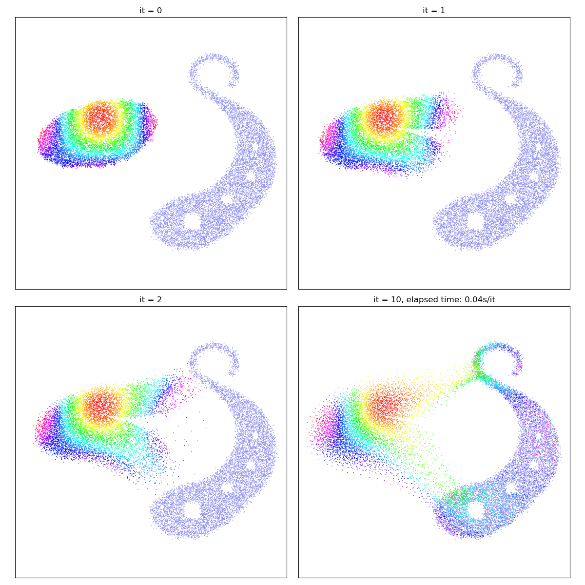
The reach parameter allows us to introduce laziness into the classical Monge problem, specifying a maximum scale (half-life) of interaction between the \(x_i\)’s and the \(y_j\)’s. It may be useful in situations where outliers are common, as it limits the influence of samples that are too far away.

gradient_descent(SamplesLoss("sinkhorn", p=2, blur=0.01, reach=0.1))

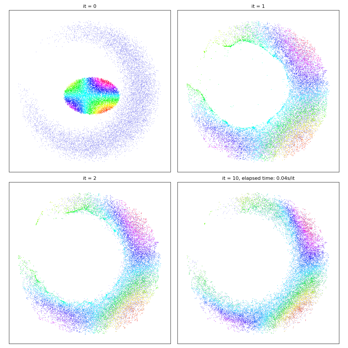
Optimal Transport is not the panacea

Optimal Transport theory is all about discarding the topological structure of the data to get a simple, convex registration algorithm: the Monge map transports bags of sands from one location to another, and may tear shapes apart as needed.

In generative modelling, this versatility allows us to fit “Gaussian blobs” to any kind of empirical distribution:

X_i = draw_samples("data/crescent_a.png", N, dtype)
Y_j = draw_samples("data/crescent_b.png", M, dtype)
gradient_descent(SamplesLoss("sinkhorn", p=2, blur=0.01))

/home/code/geomloss/geomloss/examples/optimal_transport/plot_optimal_transport_2D.py:33: DeprecationWarning: Starting with ImageIO v3 the behavior of this function will switch to that of iio.v3.imread. To keep the current behavior (and make this warning disappear) use `import imageio.v2 as imageio` or call `imageio.v2.imread` directly.
  img = imread(fname, as_gray=True)  # Grayscale

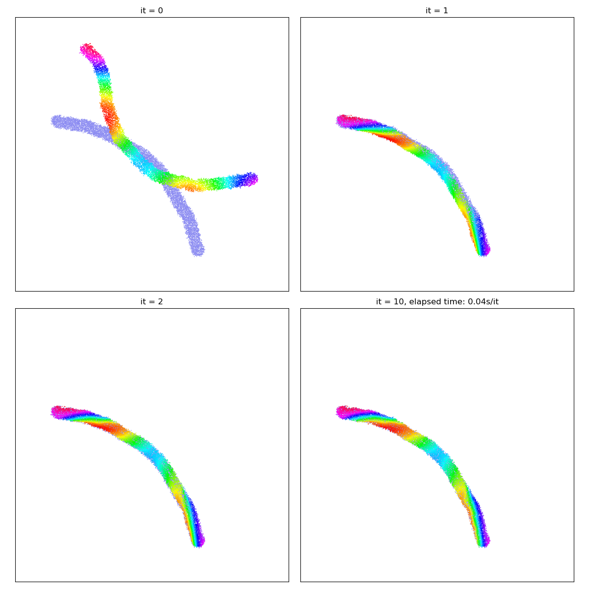
Going further, in simple situations, Optimal Transport may even be used as a “cheap and easy” registration routine…

X_i = draw_samples("data/worm_a.png", N, dtype)
Y_j = draw_samples("data/worm_b.png", M, dtype)
gradient_descent(SamplesLoss("sinkhorn", p=2, blur=0.01))

/home/code/geomloss/geomloss/examples/optimal_transport/plot_optimal_transport_2D.py:33: DeprecationWarning: Starting with ImageIO v3 the behavior of this function will switch to that of iio.v3.imread. To keep the current behavior (and make this warning disappear) use `import imageio.v2 as imageio` or call `imageio.v2.imread` directly.
  img = imread(fname, as_gray=True)  # Grayscale

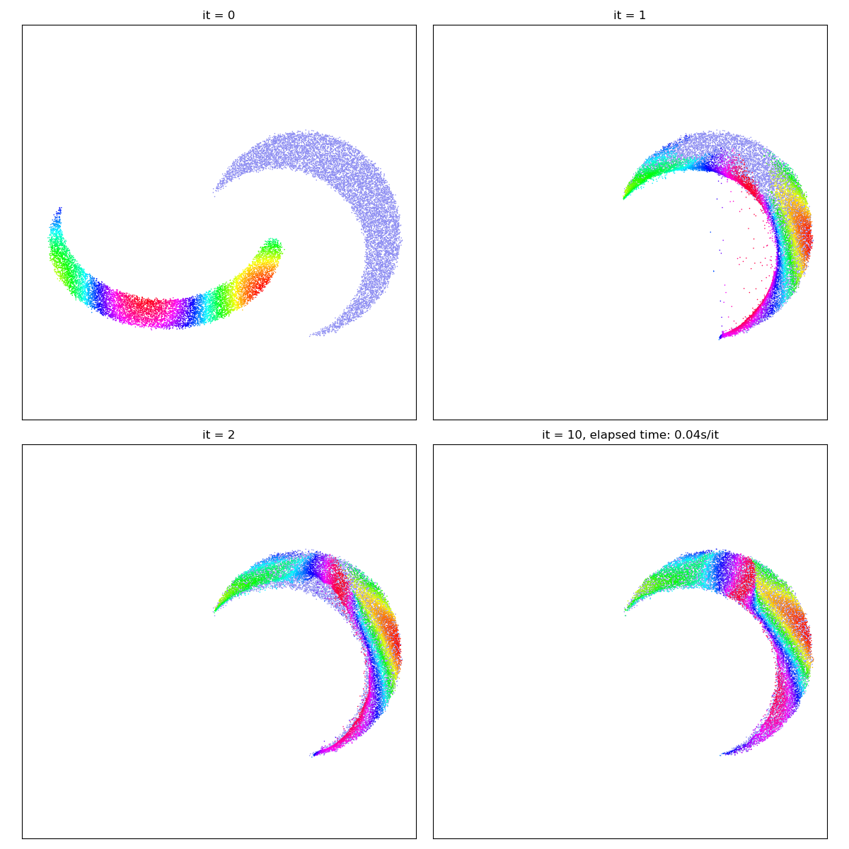
But beware! Out-of-the-box, Optimal Transport will not match the salient features of both shapes (e.g. ends or corners) with each other. In real-life applications, Sinkhorn divergences should thus always be used in a relevant feature space (e.g. of SIFT descriptors), in conjunction with a prior-enforcing generative model (e.g. a convolutional neural network or a thin plate spline deformation).

X_i = draw_samples("data/moon_a.png", N, dtype)
Y_j = draw_samples("data/moon_b.png", M, dtype)
gradient_descent(SamplesLoss("sinkhorn", p=2, blur=0.01))

plt.show()

/home/code/geomloss/geomloss/examples/optimal_transport/plot_optimal_transport_2D.py:33: DeprecationWarning: Starting with ImageIO v3 the behavior of this function will switch to that of iio.v3.imread. To keep the current behavior (and make this warning disappear) use `import imageio.v2 as imageio` or call `imageio.v2.imread` directly.
  img = imread(fname, as_gray=True)  # Grayscale