Wasserstein distances between large point clouds

Let’s compare the performances of several OT solvers on subsampled versions of the Stanford dragon, a standard test surface made up of more than 870,000 triangles. In this benchmark, we measure timings on a simple registration task: the optimal transport of a sphere onto the (subsampled) dragon, using a quadratic ground cost \(\text{C}(x,y) = \tfrac{1}{2}\|x-y\|^2\) in the ambient space \(\mathbb{R}^3\).

More precisely: having loaded and represented our 3D meshes as discrete probability measures

\[\alpha ~=~ \sum_{i=1}^N \alpha_i\,\delta_{x_i}, ~~~ \beta ~=~ \sum_{j=1}^M \beta_j\,\delta_{y_j},\]

with one weighted Dirac mass per triangle, we will strive to solve the primal-dual entropic OT problem:

\[\begin{split}\text{OT}_\varepsilon(\alpha,\beta)~&=~ \min_{0 \leqslant \pi \ll \alpha\otimes\beta} ~\langle\text{C},\pi\rangle ~+~\varepsilon\,\text{KL}(\pi,\alpha\otimes\beta) \quad\text{s.t.}~~ \pi\,\mathbf{1} = \alpha ~~\text{and}~~ \pi^\intercal \mathbf{1} = \beta\\ &=~ \max_{f,g} ~~\langle \alpha,f\rangle + \langle \beta,g\rangle - \varepsilon\langle \alpha\otimes\beta, \exp \tfrac{1}{\varepsilon}[ f\oplus g - \text{C} ] - 1 \rangle\end{split}\]

as fast as possible, optimizing on dual vectors:

\[F_i ~=~ f(x_i), ~~~ G_j ~=~ g(y_j)\]

that encode an implicit transport plan:

\[\begin{split}\pi ~&=~ \exp \tfrac{1}{\varepsilon}( f\oplus g - \text{C})~\cdot~ \alpha\otimes\beta,\\ \text{i.e.}~~\pi_{x_i \leftrightarrow y_j}~&=~ \exp \tfrac{1}{\varepsilon}( F_i + G_j - \text{C}(x_i,y_j))~\cdot~ \alpha_i \beta_j.\end{split}\]

Comparing OT solvers with each other

First, let’s make some standard imports:

import numpy as np
import torch

use_cuda = torch.cuda.is_available()
tensor = torch.cuda.FloatTensor if use_cuda else torch.FloatTensor
numpy = lambda x: x.detach().cpu().numpy()

from matplotlib import pyplot as plt
from mpl_toolkits.mplot3d import Axes3D

This tutorial is all about highlighting the differences between the GeomLoss solvers, packaged in the SamplesLoss module, and a standard Sinkhorn (or soft-Auction) loop.

from geomloss import SamplesLoss

Our baseline is provided by a simple Sinkhorn loop, implemented in the log-domain for the sake of numerical stability. Using the same code, we provide two backends: a tensorized PyTorch implementation (which has a quadratic memory footprint) and a scalable KeOps code (which has a linear memory footprint).

from pykeops.torch import LazyTensor


def sinkhorn_loop(a_i, x_i, b_j, y_j, blur=0.01, nits=100, backend="keops"):
    """Straightforward implementation of the Sinkhorn-IPFP-SoftAssign loop in the log domain."""

    # Compute the logarithm of the weights (needed in the softmin reduction) ---
    loga_i, logb_j = a_i.log(), b_j.log()
    loga_i, logb_j = loga_i[:, None, None], logb_j[None, :, None]

    # Compute the cost matrix C_ij = (1/2) * |x_i-y_j|^2 -----------------------
    if backend == "keops":  # C_ij is a *symbolic* LazyTensor
        x_i, y_j = LazyTensor(x_i[:, None, :]), LazyTensor(y_j[None, :, :])
        C_ij = ((x_i - y_j) ** 2).sum(-1) / 2  # (N,M,1) LazyTensor

    elif (
        backend == "pytorch"
    ):  # C_ij is a *full* Tensor, with a quadratic memory footprint
        # N.B.: The separable implementation below is slightly more efficient than:
        # C_ij = ((x_i[:,None,:] - y_j[None,:,:]) ** 2).sum(-1) / 2

        D_xx = (x_i ** 2).sum(-1)[:, None]  # (N,1)
        D_xy = x_i @ y_j.t()  # (N,D)@(D,M) = (N,M)
        D_yy = (y_j ** 2).sum(-1)[None, :]  # (1,M)
        C_ij = (D_xx + D_yy) / 2 - D_xy  # (N,M) matrix of halved squared distances

        C_ij = C_ij[:, :, None]  # reshape as a (N,M,1) Tensor

    # Setup the dual variables -------------------------------------------------
    eps = blur ** 2  # "Temperature" epsilon associated to our blurring scale
    F_i, G_j = torch.zeros_like(loga_i), torch.zeros_like(
        logb_j
    )  # (scaled) dual vectors

    # Sinkhorn loop = coordinate ascent on the dual maximization problem -------
    for _ in range(nits):
        F_i = -((-C_ij / eps + (G_j + logb_j))).logsumexp(dim=1)[:, None, :]
        G_j = -((-C_ij / eps + (F_i + loga_i))).logsumexp(dim=0)[None, :, :]

    # Return the dual vectors F and G, sampled on the x_i's and y_j's respectively:
    return eps * F_i, eps * G_j


# Create a sinkhorn_solver "layer" with the same signature as SamplesLoss:
from functools import partial

sinkhorn_solver = lambda blur, nits, backend: partial(
    sinkhorn_loop, blur=blur, nits=nits, backend=backend
)

Benchmarking loops

As usual, writing up a proper benchmark requires a lot of verbose, not-so-interesting code. For the sake of readabiliity, we abstracted such routines in a separate file where error functions, timers and Wasserstein distances are properly defined. Feel free to have a look!

from geomloss.examples.performances.benchmarks_ot_solvers import (
    benchmark_solver,
    benchmark_solvers,
)

The GeomLoss routines rely on a scaling parameter to tune the tradeoff between speed (scaling \(\rightarrow\) 0) and accuracy (scaling \(\rightarrow\) 1). Meanwhile, the Sinkhorn loop is directly controlled by a number of iterations that should be chosen with respect to the available time budget.

def full_benchmark(source, target, blur, maxtime=None):

    # Compute a suitable "ground truth" ----------------------------------------
    OT_solver = SamplesLoss(
        "sinkhorn",
        p=2,
        blur=blur,
        backend="online",
        scaling=0.999,
        debias=False,
        potentials=True,
    )
    _, _, ground_truth = benchmark_solver(OT_solver, blur, sources[0], targets[0])

    results = {}  # Dict of "timings vs errors" arrays

    # Compute statistics for the three backends of GeomLoss: -------------------

    for name in ["multiscale-1", "multiscale-5", "online", "tensorized"]:
        if name == "multiscale-1":
            backend, truncate = "multiscale", 1  # Aggressive "kernel truncation" scheme
        elif name == "multiscale-5":
            backend, truncate = "multiscale", 5  # Safe, default truncation rule
        else:
            backend, truncate = name, None

        OT_solvers = [
            SamplesLoss(
                "sinkhorn",
                p=2,
                blur=blur,
                scaling=scaling,
                truncate=truncate,
                backend=backend,
                debias=False,
                potentials=True,
            )
            for scaling in [0.5, 0.6, 0.7, 0.8, 0.9, 0.95, 0.99]
        ]

        results[name] = benchmark_solvers(
            "GeomLoss - " + name,
            OT_solvers,
            source,
            target,
            ground_truth,
            blur=blur,
            display=False,
            maxtime=maxtime,
        )

    # Compute statistics for a naive Sinkhorn loop -----------------------------

    for backend in ["pytorch", "keops"]:
        OT_solvers = [
            sinkhorn_solver(blur, nits=nits, backend=backend)
            for nits in [5, 10, 20, 50, 100, 200, 500, 1000, 2000, 5000, 10000]
        ]

        results[backend] = benchmark_solvers(
            "Sinkhorn loop - " + backend,
            OT_solvers,
            source,
            target,
            ground_truth,
            blur=blur,
            display=False,
            maxtime=maxtime,
        )

    return results, ground_truth

Having solved the entropic OT problem with dozens of configurations, we will display our results in an “error vs timing” log-log plot:

def display_statistics(title, results, ground_truth, maxtime=None):
    """Displays a "error vs timing" plot in log-log scale."""

    curves = [
        ("pytorch", "Sinkhorn loop - PyTorch backend"),
        ("keops", "Sinkhorn loop - KeOps backend"),
        ("tensorized", "Sinkhorn with ε-scaling - PyTorch backend"),
        ("online", "Sinkhorn with ε-scaling - KeOps backend"),
        ("multiscale-5", "Sinkhorn multiscale - truncate=5 (safe)"),
        ("multiscale-1", "Sinkhorn multiscale - truncate=1 (fast)"),
    ]

    fig = plt.figure(figsize=(12, 8))
    ax = fig.subplots()
    ax.set_title(title)
    ax.set_ylabel("Relative error made on the entropic Wasserstein distance")
    ax.set_yscale("log")
    ax.set_ylim(top=1e-1, bottom=1e-3)
    ax.set_xlabel("Time (s)")
    ax.set_xscale("log")
    ax.set_xlim(left=1e-3, right=maxtime)

    ax.grid(True, which="major", linestyle="-")
    ax.grid(True, which="minor", linestyle="dotted")

    for key, name in curves:
        timings, errors, costs = results[key]
        ax.plot(timings, np.abs(costs - ground_truth), label=name)

    ax.legend(loc="upper right")


def full_statistics(source, target, blur=0.01, maxtime=None):
    results, ground_truth = full_benchmark(source, target, blur, maxtime=maxtime)

    display_statistics(
        "Solving a {:,}-by-{:,} OT problem, with a blurring scale σ = {:}".format(
            len(source[0]), len(target[0]), blur
        ),
        results,
        ground_truth,
        maxtime=maxtime,
    )

    return results, ground_truth

Building our dataset

Our source measures: unit spheres, sampled with (roughly) the same number of points as the target meshes:

from geomloss.examples.performances.benchmarks_ot_solvers import create_sphere

sources = [create_sphere(npoints) for npoints in [1e4, 5e4, 2e5, 8e5]]

Then, we fetch our target models from the Stanford repository:

import os

if not os.path.exists("data/dragon_recon/dragon_vrip_res4.ply"):
    import urllib.request

    urllib.request.urlretrieve(
        "http://graphics.stanford.edu/pub/3Dscanrep/dragon/dragon_recon.tar.gz",
        "data/dragon.tar.gz",
    )

    import shutil

    shutil.unpack_archive("data/dragon.tar.gz", "data")

To read the raw .ply ascii files, we rely on the plyfile package:

from geomloss.examples.performances.benchmarks_ot_solvers import (
    load_ply_file,
    display_cloud,
)

Our meshes are encoded using one weighted Dirac mass per triangle. To keep things simple, we use as targets the subsamplings provided in the reference Stanford archive. Feel free to re-run this script with your own models!

# N.B.: Since Plyfile is far from being optimized, this may take some time!
targets = [
    load_ply_file(fname, offset=[-0.011, 0.109, -0.008], scale=0.04)
    for fname in [
        "data/dragon_recon/dragon_vrip_res4.ply",  # ~ 10,000 triangles
        "data/dragon_recon/dragon_vrip_res3.ply",  # ~ 50,000 triangles
        "data/dragon_recon/dragon_vrip_res2.ply",  # ~200,000 triangles
        #'data/dragon_recon/dragon_vrip.ply',     # ~800,000 triangles
    ]
]

File loaded, and encoded as the weighted sum of 11,102 atoms in 3D.
File loaded, and encoded as the weighted sum of 47,794 atoms in 3D.
File loaded, and encoded as the weighted sum of 202,520 atoms in 3D.

Finally, if we don’t have access to a GPU, we subsample point clouds while making sure that weights still sum up to one:

def subsample(measure, decimation=500):
    weights, locations = measure
    weights, locations = weights[::decimation], locations[::decimation]
    weights = weights / weights.sum()
    return weights.contiguous(), locations.contiguous()


if not use_cuda:
    sources = [subsample(s) for s in sources]
    targets = [subsample(t) for t in targets]

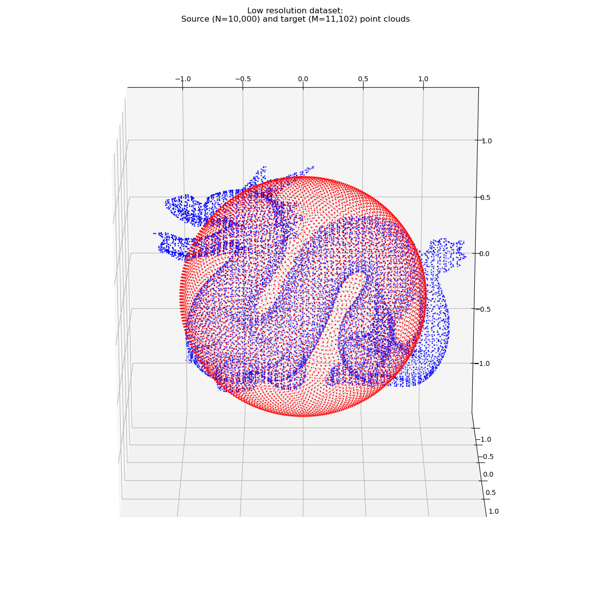
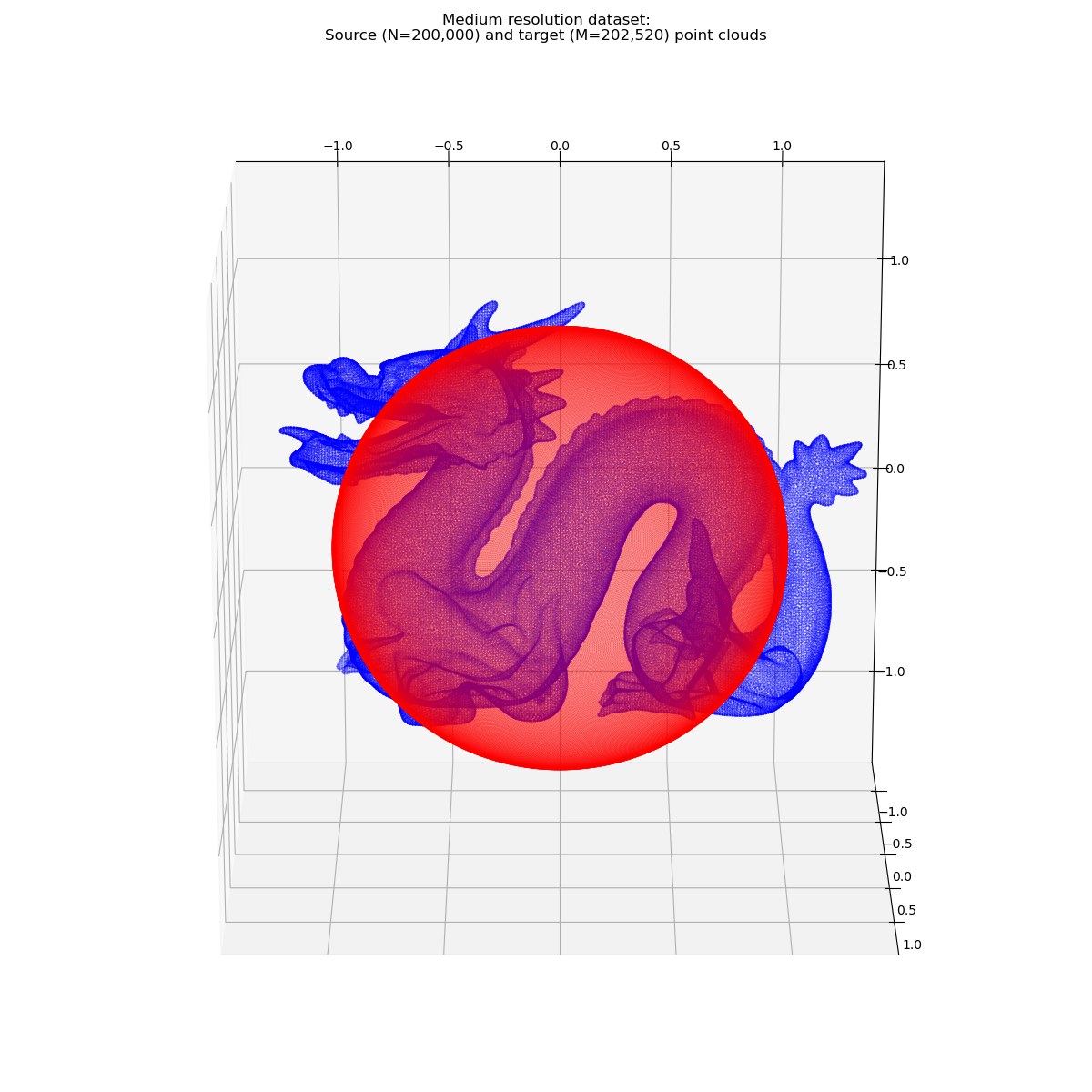
In this simple benchmark, we will only use the coarse and medium resolutions of our meshes: 200,000 points should be more than enough to compute sensible approximations of the Wasserstein distance between the Stanford dragon and a unit sphere!

fig = plt.figure(figsize=(12, 12))
ax = fig.add_subplot(1, 1, 1, projection="3d")
display_cloud(ax, sources[0], "red")
display_cloud(ax, targets[0], "blue")
ax.set_title(
    "Low resolution dataset:\n"
    + "Source (N={:,}) and target (M={:,}) point clouds".format(
        len(sources[0][0]), len(targets[0][0])
    )
)
plt.tight_layout()

# sphinx_gallery_thumbnail_number = 2
fig = plt.figure(figsize=(12, 12))
ax = fig.add_subplot(1, 1, 1, projection="3d")
display_cloud(ax, sources[2], "red")
display_cloud(ax, targets[2], "blue")
ax.set_title(
    "Medium resolution dataset:\n"
    + "Source (N={:,}) and target (M={:,}) point clouds".format(
        len(sources[2][0]), len(targets[2][0])
    )
)
plt.tight_layout()

• 
• 

Benchmarks

Choosing a temperature. Understood as a smooth generalization of the standard theory of auctions, entropic regularization allows us to compute tractable approximations of the Wasserstein distance on the GPU.

The level of approximation is set using a single parameter, the temperature \(\varepsilon > 0\) which is homogeneous to the cost function \(\text{C}\): with a number of iterations that scales roughly in

\[\begin{split}\begin{cases} O \Big( \frac{ \max_{i,j}\text{C}(x_i,y_j) }{ \varepsilon } \Big) & \text{with the Sinkhorn and Auction algorithms} \\ O \Big( \log \Big( \frac{ \max_{i,j}\text{C}(x_i,y_j) }{ \varepsilon } \Big) \Big) & \text{using an $\varepsilon$-scaling annealing strategy,} \end{cases}\end{split}\]

we may compute an approximation \(\text{OT}_\varepsilon\) of the transport cost with precision \(\simeq \varepsilon\).

Choosing a blurring scale. In practice, when \(\text{C}(x,y) = \tfrac{1}{p}\|x-y\|^p\) is the standard Wasserstein cost, the temperature \(\varepsilon\) is best understood through its p-th root:

\[\sigma ~=~ \sqrt[p]{\varepsilon},\]

the blurring scale of the (Laplacian if p=1, Gaussian if p=2) Gibbs kernel

\[k_\varepsilon(x,y) ~=~ \exp(-\text{C}(x,y)/\varepsilon)\]

through which the Sinkhorn algorithm interacts with our weighted point clouds. According to the heuristics presented above, we may thus expect to solve a regularized \(\text{OT}_\varepsilon\) problem in

\[\begin{split}\begin{cases} O \big( ( \text{D} / \sigma )^p \big) & \text{with the Sinkhorn and Auction algorithms} \\ O \big( \log ( \text{D} / \sigma ) \big) & \text{using an $\varepsilon$-scaling annealing strategy,} \end{cases}\end{split}\]

with \(\text{D} = \max_{i,j}\|x_i-y_j\|\) the diameter of our configuration. We now focus on the case where p=2, which provides the most useful gradients in geometric shape analysis, and discuss the performances of our routines as we change the blurring scale \(\sigma = \sqrt{\varepsilon}\) and the number of samples \(\sqrt{MN}\).

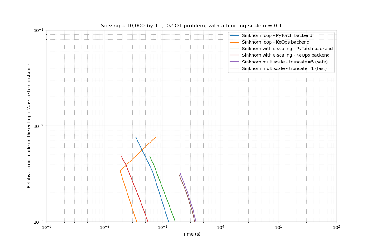
High-temperature OT

Cuturi-like setting. A current trend in Machine Learning is to rely on large blurring scales to compute low-resolution gradients: giving up on precision is understood as a way of becoming robust to sampling noise in high dimensions.

Judging from the pictures above, the Wasserstein distance between our unit sphere and the Stanford dragon should be of order 1 and most likely close to 0.5. Consequently, a blurring scale set to \(\sigma = \texttt{0.1}\), that corresponds to a temperature \(\varepsilon = \sigma^p = \texttt{0.01}\), should allow us to emulate the typical regime of the current Machine Learning literature.

maxtime = 100 if use_cuda else 1

full_statistics(sources[0], targets[0], blur=0.10, maxtime=maxtime)

Benchmarking the "GeomLoss - multiscale-1" family of OT solvers - ground truth = 0.560432:
1-th solver : t = 0.1923, error on the constraints = 0.261, cost = 0.557364
2-th solver : t = 0.1927, error on the constraints = 0.295, cost = 0.557379
3-th solver : t = 0.2557, error on the constraints = 0.090, cost = 0.558416
4-th solver : t = 0.3191, error on the constraints = 0.071, cost = 0.559113
5-th solver : t = 0.4501, error on the constraints = 0.046, cost = 0.559866
6-th solver : t = 0.8546, error on the constraints = 0.027, cost = 0.560243
7-th solver : t = 3.8760, error on the constraints = 0.006, cost = 0.560432

Benchmarking the "GeomLoss - multiscale-5" family of OT solvers - ground truth = 0.560432:
1-th solver : t = 0.2013, error on the constraints = 0.123, cost = 0.557271
2-th solver : t = 0.2010, error on the constraints = 0.113, cost = 0.557242
3-th solver : t = 0.2677, error on the constraints = 0.090, cost = 0.558409
4-th solver : t = 0.3343, error on the constraints = 0.071, cost = 0.559108
5-th solver : t = 0.4704, error on the constraints = 0.046, cost = 0.559849
6-th solver : t = 0.8719, error on the constraints = 0.027, cost = 0.560227
7-th solver : t = 3.8865, error on the constraints = 0.006, cost = 0.560422

Benchmarking the "GeomLoss - online" family of OT solvers - ground truth = 0.560432:
1-th solver : t = 0.0194, error on the constraints = 0.260, cost = 0.555675
2-th solver : t = 0.0232, error on the constraints = 0.169, cost = 0.556500
3-th solver : t = 0.0289, error on the constraints = 0.120, cost = 0.557635
4-th solver : t = 0.0404, error on the constraints = 0.083, cost = 0.558731
5-th solver : t = 0.0730, error on the constraints = 0.048, cost = 0.559797
6-th solver : t = 0.1256, error on the constraints = 0.026, cost = 0.560236
7-th solver : t = 0.6075, error on the constraints = 0.006, cost = 0.560422

Benchmarking the "GeomLoss - tensorized" family of OT solvers - ground truth = 0.560432:
1-th solver : t = 0.0600, error on the constraints = 0.260, cost = 0.555675
2-th solver : t = 0.0700, error on the constraints = 0.169, cost = 0.556500
3-th solver : t = 0.0862, error on the constraints = 0.120, cost = 0.557636
4-th solver : t = 0.1187, error on the constraints = 0.083, cost = 0.558731
5-th solver : t = 0.2163, error on the constraints = 0.048, cost = 0.559797
6-th solver : t = 0.4166, error on the constraints = 0.026, cost = 0.560236
7-th solver : t = 1.9924, error on the constraints = 0.006, cost = 0.560422

Benchmarking the "Sinkhorn loop - pytorch" family of OT solvers - ground truth = 0.560432:
1-th solver : t = 0.0342, error on the constraints = 0.141, cost = 0.552788
2-th solver : t = 0.0664, error on the constraints = 0.080, cost = 0.557057
3-th solver : t = 0.1308, error on the constraints = 0.038, cost = 0.559497
4-th solver : t = 0.3240, error on the constraints = 0.008, cost = 0.560371
5-th solver : t = 0.6460, error on the constraints = 0.002, cost = 0.560429
6-th solver : t = 1.2905, error on the constraints = 0.000, cost = 0.560432
7-th solver : t = 3.2227, error on the constraints = 0.000, cost = 0.560432
8-th solver : t = 6.4442, error on the constraints = 0.000, cost = 0.560432
9-th solver : t = 12.8866, error on the constraints = 0.000, cost = 0.560432
10-th solver : t = 32.2117, error on the constraints = 0.000, cost = 0.560432
11-th solver : t = 64.4231, error on the constraints = 0.000, cost = 0.560432

Benchmarking the "Sinkhorn loop - keops" family of OT solvers - ground truth = 0.560432:
1-th solver : t = 0.0762, error on the constraints = 0.141, cost = 0.552788
2-th solver : t = 0.0184, error on the constraints = 0.080, cost = 0.557057
3-th solver : t = 0.0367, error on the constraints = 0.038, cost = 0.559497
4-th solver : t = 0.0915, error on the constraints = 0.008, cost = 0.560371
5-th solver : t = 0.1824, error on the constraints = 0.002, cost = 0.560429
6-th solver : t = 0.3650, error on the constraints = 0.000, cost = 0.560432
7-th solver : t = 0.9112, error on the constraints = 0.000, cost = 0.560432
8-th solver : t = 1.8244, error on the constraints = 0.000, cost = 0.560432
9-th solver : t = 3.6480, error on the constraints = 0.000, cost = 0.560432
10-th solver : t = 9.1202, error on the constraints = 0.000, cost = 0.560432
11-th solver : t = 18.2411, error on the constraints = 0.000, cost = 0.560432


({'multiscale-1': (array([0.19229484, 0.19270444, 0.25571299, 0.31913781, 0.45013666,
       0.85457373, 3.87599754]), array([0.26076049, 0.2952348 , 0.08960721, 0.07076597, 0.04605597,
       0.02667859, 0.0062393 ]), array([0.5573644 , 0.55737931, 0.55841631, 0.55911314, 0.55986607,
       0.56024343, 0.56043231])), 'multiscale-5': (array([0.20134425, 0.20100474, 0.26772714, 0.33432603, 0.47037101,
       0.87185383, 3.88654494]), array([0.12280504, 0.11253369, 0.08969046, 0.07090178, 0.04620221,
       0.02672147, 0.00594249]), array([0.55727118, 0.55724192, 0.5584088 , 0.55910838, 0.55984944,
       0.56022739, 0.56042194])), 'online': (array([0.01938343, 0.02318048, 0.02890468, 0.04037714, 0.07297182,
       0.12560058, 0.60750699]), array([0.25995392, 0.16854914, 0.12009196, 0.08318655, 0.04838723,
       0.02601784, 0.00584987]), array([0.55567539, 0.5564999 , 0.55763549, 0.55873132, 0.55979651,
       0.56023645, 0.56042194])), 'tensorized': (array([0.05998564, 0.07001042, 0.08623552, 0.11873913, 0.21625853,
       0.41660619, 1.99237418]), array([0.25995365, 0.16854897, 0.12009189, 0.08318652, 0.04838721,
       0.02601783, 0.00584986]), array([0.55567539, 0.55649984, 0.55763555, 0.55873126, 0.55979657,
       0.56023645, 0.56042194])), 'pytorch': (array([3.41753960e-02, 6.63599968e-02, 1.30836248e-01, 3.24028730e-01,
       6.46038294e-01, 1.29045844e+00, 3.22271895e+00, 6.44423890e+00,
       1.28865590e+01, 3.22117038e+01, 6.44230978e+01]), array([1.40665218e-01, 8.03463757e-02, 3.80394384e-02, 7.57312402e-03,
       1.53424859e-03, 1.33747715e-04, 7.94345283e-07, 7.11446148e-07,
       7.06059154e-07, 7.05596847e-07, 7.02678108e-07]), array([0.55278832, 0.55705744, 0.55949718, 0.56037122, 0.56042886,
       0.5604322 , 0.5604322 , 0.5604322 , 0.5604322 , 0.5604322 ,
       0.5604322 ])), 'keops': (array([ 0.07618523,  0.0184257 ,  0.03670239,  0.0915041 ,  0.18239617,
        0.36502957,  0.91116667,  1.82440329,  3.64801669,  9.12021136,
       18.2410562 ]), array([1.40665025e-01, 8.03461745e-02, 3.80392149e-02, 7.57289119e-03,
       1.53401692e-03, 1.33516514e-04, 4.35923482e-07, 2.98747352e-07,
       2.98590635e-07, 2.96990834e-07, 2.95383757e-07]), array([0.55278832, 0.5570575 , 0.55949718, 0.56037122, 0.56042886,
       0.5604322 , 0.5604322 , 0.5604322 , 0.5604322 , 0.5604322 ,
       0.5604322 ]))}, 0.5604320764541626)

Breakdown of the results. When the diameter-to-blur ratio \(D/\sigma\) is of order 10, as is often the case in ML, the baseline Sinkhorn algorithm works just fine.

As discussed in our AiStats 2019 paper, improvements in this regime mostly come down to a clever low-level implementation of the SoftMin reduction, abstracted in the KeOps library: Switching from PyTorch to KeOps allows us to get a x10 speed-up and break the memory bottleneck, but scaling strategies are overkill for this simple, low-resolution problem.

Note

When

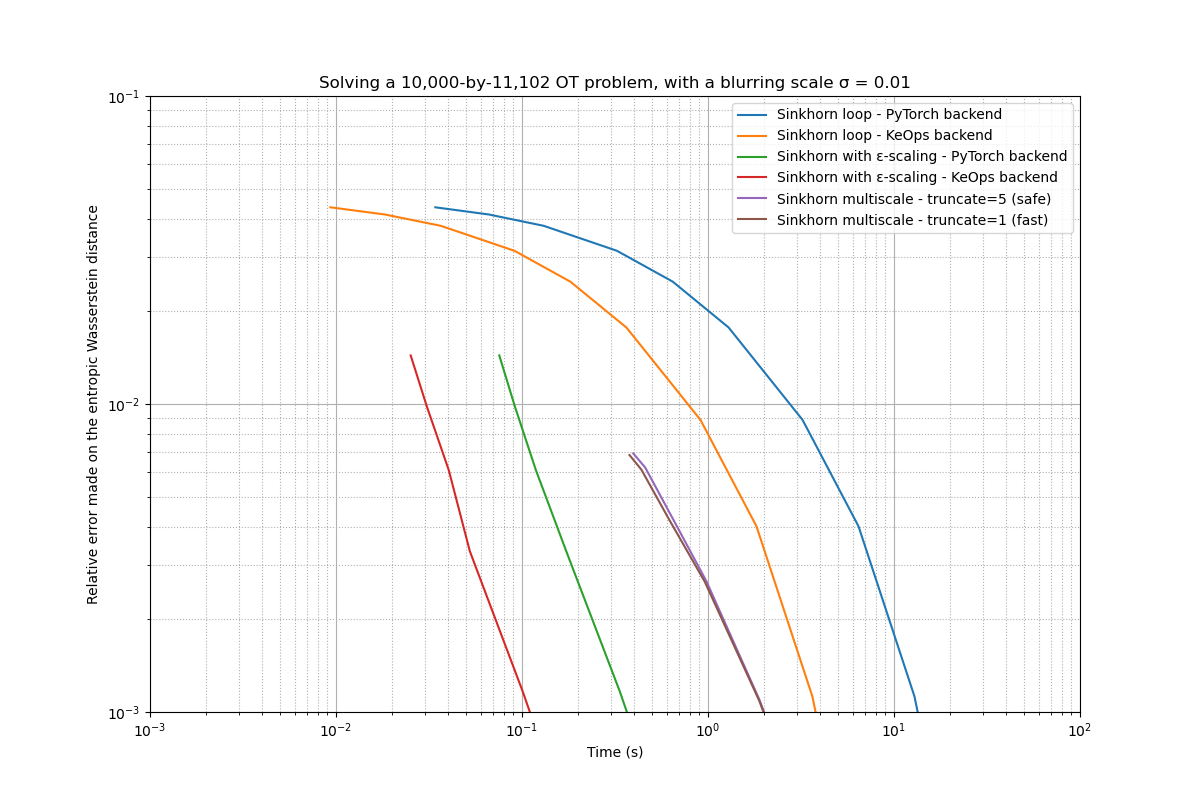
Low-temperature OT

Graphics-like setting. Keep in mind, though, that the performances of the baseline Sinkhorn loop completely break down as we try to reduce our blurring scale \(\sigma\). In Computer Graphics and Medical Imaging, a realistic use-case is to pick a diameter-to-blur ratio \(D/\sigma\) of order 100, which lets us take into account the detailed features of our shapes: for normalized point clouds, a value of \(\sigma = \texttt{0.01}\) – that corresponds to a temperature \(\varepsilon = \sigma^p = \texttt{0.0001}\) – is a sensible pick.

full_statistics(sources[0], targets[0], blur=0.01, maxtime=maxtime)

Benchmarking the "GeomLoss - multiscale-1" family of OT solvers - ground truth = 0.468990:
1-th solver : t = 0.3783, error on the constraints = nan, cost = 0.462160
2-th solver : t = 0.4381, error on the constraints = nan, cost = 0.462864
3-th solver : t = 0.6242, error on the constraints = 0.239, cost = 0.464819
4-th solver : t = 0.9601, error on the constraints = 0.156, cost = 0.466339
5-th solver : t = 1.8831, error on the constraints = 16.101, cost = 0.467900
6-th solver : t = 3.6924, error on the constraints = 3.776, cost = 0.468620
7-th solver : t = 18.6636, error on the constraints = 0.016, cost = 0.468973

Benchmarking the "GeomLoss - multiscale-5" family of OT solvers - ground truth = 0.468990:
1-th solver : t = 0.3963, error on the constraints = 1.757, cost = 0.462076
2-th solver : t = 0.4594, error on the constraints = 0.391, cost = 0.462769
3-th solver : t = 0.6566, error on the constraints = 0.239, cost = 0.464817
4-th solver : t = 0.9816, error on the constraints = 0.156, cost = 0.466336
5-th solver : t = 1.8936, error on the constraints = 0.096, cost = 0.467896
6-th solver : t = 3.7072, error on the constraints = 0.058, cost = 0.468618
7-th solver : t = 18.7347, error on the constraints = 0.016, cost = 0.468973

Benchmarking the "GeomLoss - online" family of OT solvers - ground truth = 0.468990:
1-th solver : t = 0.0252, error on the constraints = 39.021, cost = 0.454610
2-th solver : t = 0.0308, error on the constraints = 0.656, cost = 0.459198
3-th solver : t = 0.0404, error on the constraints = 0.301, cost = 0.462893
4-th solver : t = 0.0524, error on the constraints = 0.170, cost = 0.465662
5-th solver : t = 0.1008, error on the constraints = 0.097, cost = 0.467822
6-th solver : t = 0.1984, error on the constraints = 0.058, cost = 0.468628
7-th solver : t = 0.9847, error on the constraints = 0.016, cost = 0.468972

Benchmarking the "GeomLoss - tensorized" family of OT solvers - ground truth = 0.468990:
1-th solver : t = 0.0755, error on the constraints = 39.001, cost = 0.454610
2-th solver : t = 0.0917, error on the constraints = 0.656, cost = 0.459198
3-th solver : t = 0.1188, error on the constraints = 0.301, cost = 0.462893
4-th solver : t = 0.1729, error on the constraints = 0.170, cost = 0.465662
5-th solver : t = 0.3354, error on the constraints = 0.097, cost = 0.467822
6-th solver : t = 0.6548, error on the constraints = 0.058, cost = 0.468628
7-th solver : t = 3.2323, error on the constraints = 0.016, cost = 0.468972

Benchmarking the "Sinkhorn loop - pytorch" family of OT solvers - ground truth = 0.468990:
1-th solver : t = 0.0342, error on the constraints = 1.452, cost = 0.425475
2-th solver : t = 0.0664, error on the constraints = 1.114, cost = 0.427754
3-th solver : t = 0.1308, error on the constraints = 0.801, cost = 0.431099
4-th solver : t = 0.3241, error on the constraints = 0.518, cost = 0.437559
5-th solver : t = 0.6462, error on the constraints = 0.377, cost = 0.444029
6-th solver : t = 1.2903, error on the constraints = 0.261, cost = 0.451269
7-th solver : t = 3.2231, error on the constraints = 0.144, cost = 0.460108
8-th solver : t = 6.4444, error on the constraints = 0.083, cost = 0.464981
9-th solver : t = 12.8871, error on the constraints = 0.039, cost = 0.467867
10-th solver : t = 32.2144, error on the constraints = 0.008, cost = 0.468915
11-th solver : t = 64.4216, error on the constraints = 0.002, cost = 0.468986

Benchmarking the "Sinkhorn loop - keops" family of OT solvers - ground truth = 0.468990:
1-th solver : t = 0.0093, error on the constraints = 1.452, cost = 0.425475
2-th solver : t = 0.0183, error on the constraints = 1.114, cost = 0.427754
3-th solver : t = 0.0366, error on the constraints = 0.801, cost = 0.431099
4-th solver : t = 0.0911, error on the constraints = 0.518, cost = 0.437559
5-th solver : t = 0.1819, error on the constraints = 0.377, cost = 0.444029
6-th solver : t = 0.3641, error on the constraints = 0.261, cost = 0.451269
7-th solver : t = 0.9108, error on the constraints = 0.144, cost = 0.460108
8-th solver : t = 1.8222, error on the constraints = 0.083, cost = 0.464981
9-th solver : t = 3.6413, error on the constraints = 0.039, cost = 0.467867
10-th solver : t = 9.1024, error on the constraints = 0.008, cost = 0.468915
11-th solver : t = 18.2311, error on the constraints = 0.002, cost = 0.468986


({'multiscale-1': (array([ 0.37828302,  0.43810797,  0.62420654,  0.96006107,  1.88313246,
        3.69244242, 18.66364479]), array([           nan,            nan, 2.38995865e-01, 1.56047225e-01,
       1.61012936e+01, 3.77588296e+00, 1.55185964e-02]), array([0.46216008, 0.4628644 , 0.46481892, 0.46633887, 0.46789977,
       0.46862018, 0.46897259])), 'multiscale-5': (array([ 0.39630294,  0.45942831,  0.65661883,  0.98156047,  1.89364409,
        3.70724535, 18.73466778]), array([1.75681281, 0.39094663, 0.23930818, 0.15618092, 0.09587701,
       0.05807068, 0.01552475]), array([0.46207568, 0.46276882, 0.46481746, 0.46633554, 0.46789643,
       0.46861839, 0.46897256])), 'online': (array([0.02520871, 0.03083062, 0.04040194, 0.05241632, 0.10080576,
       0.19837284, 0.9847455 ]), array([3.90209427e+01, 6.55859709e-01, 3.01485807e-01, 1.70306653e-01,
       9.72800478e-02, 5.77253550e-02, 1.55339884e-02]), array([0.45461038, 0.45919755, 0.46289313, 0.46566191, 0.46782231,
       0.46862802, 0.46897218])), 'tensorized': (array([0.07547903, 0.09169316, 0.11880422, 0.17293739, 0.33536935,
       0.65478992, 3.23227143]), array([3.90007820e+01, 6.55819058e-01, 3.01475048e-01, 1.70304835e-01,
       9.72797275e-02, 5.77267855e-02, 1.55369919e-02]), array([0.45461035, 0.45919755, 0.4628931 , 0.46566194, 0.46782231,
       0.46862802, 0.46897215])), 'pytorch': (array([3.41989994e-02, 6.63878918e-02, 1.30781889e-01, 3.24107647e-01,
       6.46239281e-01, 1.29029703e+00, 3.22308707e+00, 6.44442821e+00,
       1.28871214e+01, 3.22143564e+01, 6.44215593e+01]), array([1.45177937, 1.11441219, 0.80101037, 0.51840079, 0.37667969,
       0.26148966, 0.14429921, 0.08290579, 0.03945083, 0.00801208,
       0.00176246]), array([0.42547518, 0.42775351, 0.43109873, 0.43755883, 0.44402876,
       0.4512693 , 0.46010789, 0.46498132, 0.46786666, 0.46891472,
       0.46898565])), 'keops': (array([9.32121277e-03, 1.83234215e-02, 3.65769863e-02, 9.11440849e-02,
       1.81871414e-01, 3.64076138e-01, 9.10807371e-01, 1.82219839e+00,
       3.64126468e+00, 9.10242176e+00, 1.82311141e+01]), array([1.45174754, 1.11434102, 0.8009215 , 0.51827741, 0.3765409 ,
       0.26135418, 0.14416541, 0.08277068, 0.03931752, 0.00787629,
       0.00162181]), array([0.42547518, 0.42775351, 0.43109873, 0.43755883, 0.44402879,
       0.4512693 , 0.46010792, 0.46498135, 0.46786666, 0.46891472,
       0.46898565]))}, 0.4689895510673523)

Breakdown of the results. As expected, dividing by ten the blurring scale \(\sigma\) leads to a 100-fold increase in the number of iterations needed by the (simple) Sinkhorn loop… whereas routines that relied on \(\varepsilon\)-scaling only experienced a 2-fold slow-down! Well documented for entropic OT since the 90’s, the use of annealing strategies is thus critical as soon as some level of accuracy is required.

Going further, adaptive clustering strategies allow us to break the \(O(NM)\) complexity of exact SoftMin reductions, as discussed in previous tutorials:

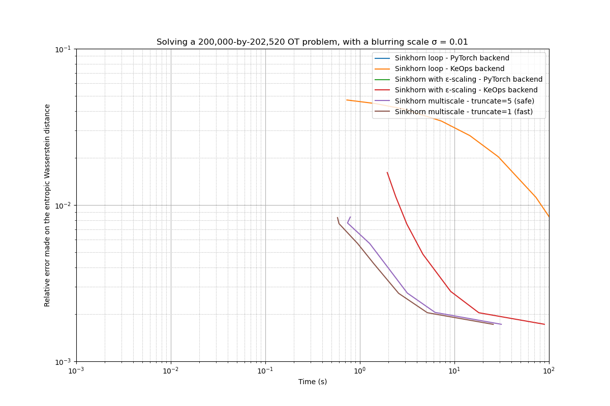
full_statistics(sources[2], targets[2], blur=0.01, maxtime=maxtime)

Benchmarking the "GeomLoss - multiscale-1" family of OT solvers - ground truth = 0.468990:
1-th solver : t = 0.5797, error on the constraints = nan, cost = 0.460679
2-th solver : t = 0.6011, error on the constraints = nan, cost = 0.461384
3-th solver : t = 0.9475, error on the constraints = nan, cost = 0.463323
4-th solver : t = 1.4061, error on the constraints = nan, cost = 0.464781
5-th solver : t = 2.5686, error on the constraints = nan, cost = 0.466266
6-th solver : t = 5.1702, error on the constraints = nan, cost = 0.466942
7-th solver : t = 25.7228, error on the constraints = nan, cost = 0.467265

Benchmarking the "GeomLoss - multiscale-5" family of OT solvers - ground truth = 0.468990:
1-th solver : t = 0.7909, error on the constraints = 1.284, cost = 0.460613
2-th solver : t = 0.7391, error on the constraints = 0.321, cost = 0.461309
3-th solver : t = 1.2703, error on the constraints = 0.211, cost = 0.463319
4-th solver : t = 1.8446, error on the constraints = 0.140, cost = 0.464776
5-th solver : t = 3.1744, error on the constraints = 0.081, cost = 0.466257
6-th solver : t = 6.2505, error on the constraints = 0.045, cost = 0.466935
7-th solver : t = 31.3016, error on the constraints = 0.010, cost = 0.467263

Benchmarking the "GeomLoss - online" family of OT solvers - ground truth = 0.468990:
1-th solver : t = 1.9457, error on the constraints = 14.010, cost = 0.452836
2-th solver : t = 2.3945, error on the constraints = 0.591, cost = 0.457689
3-th solver : t = 3.1427, error on the constraints = 0.275, cost = 0.461453
4-th solver : t = 4.6388, error on the constraints = 0.155, cost = 0.464145
5-th solver : t = 9.1277, error on the constraints = 0.083, cost = 0.466189
6-th solver : t = 18.1074, error on the constraints = 0.045, cost = 0.466943
7-th solver : t = 89.3400, error on the constraints = 0.010, cost = 0.467263

Benchmarking the "GeomLoss - tensorized" family of OT solvers - ground truth = 0.468990:
** Memory overflow ! **

Benchmarking the "Sinkhorn loop - pytorch" family of OT solvers - ground truth = 0.468990:
** Memory overflow ! **

Benchmarking the "Sinkhorn loop - keops" family of OT solvers - ground truth = 0.468990:
1-th solver : t = 0.7284, error on the constraints = 1.493, cost = 0.421998
2-th solver : t = 1.4549, error on the constraints = 1.072, cost = 0.424401
3-th solver : t = 2.9092, error on the constraints = 0.767, cost = 0.427872
4-th solver : t = 7.2715, error on the constraints = 0.516, cost = 0.434530
5-th solver : t = 14.5433, error on the constraints = 0.379, cost = 0.441180
6-th solver : t = 29.0883, error on the constraints = 0.265, cost = 0.448629
7-th solver : t = 72.7411, error on the constraints = 0.148, cost = 0.457788
8-th solver : t = 145.5403, error on the constraints = 0.086, cost = 0.462946


({'multiscale-1': (array([ 0.57965207,  0.60105062,  0.94748569,  1.40609121,  2.56856012,
        5.17015719, 25.72284222]), array([nan, nan, nan, nan, nan, nan, nan]), array([0.46067929, 0.46138445, 0.46332318, 0.46478114, 0.46626619,
       0.46694231, 0.46726525])), 'multiscale-5': (array([ 0.79085946,  0.73913264,  1.27033615,  1.84459162,  3.17438197,
        6.25054479, 31.30164742]), array([1.28350472, 0.32087588, 0.21082613, 0.13982332, 0.08148508,
       0.04524117, 0.0095937 ]), array([0.46061343, 0.46130911, 0.46331888, 0.46477553, 0.46625695,
       0.46693456, 0.46726319])), 'online': (array([ 1.94566202,  2.3945148 ,  3.1426816 ,  4.63879776,  9.12773514,
       18.10735488, 89.34000134]), array([1.40100918e+01, 5.90899229e-01, 2.74631292e-01, 1.54590964e-01,
       8.32118765e-02, 4.48429435e-02, 9.59692802e-03]), array([0.45283607, 0.45768943, 0.46145335, 0.46414521, 0.46618912,
       0.4669432 , 0.46726292])), 'tensorized': (array([nan, nan, nan, nan, nan, nan, nan]), array([nan, nan, nan, nan, nan, nan, nan]), array([nan, nan, nan, nan, nan, nan, nan])), 'pytorch': (array([nan, nan, nan, nan, nan, nan, nan, nan, nan, nan, nan]), array([nan, nan, nan, nan, nan, nan, nan, nan, nan, nan, nan]), array([nan, nan, nan, nan, nan, nan, nan, nan, nan, nan, nan])), 'keops': (array([  0.72835279,   1.45485067,   2.90923834,   7.27154064,
        14.54330897,  29.08832979,  72.7411201 , 145.54030156,
                nan,          nan,          nan]), array([1.49341023, 1.07193971, 0.76744741, 0.51586437, 0.3786965 ,
       0.26466152, 0.14763255, 0.08564569,        nan,        nan,
              nan]), array([0.42199785, 0.42440093, 0.42787209, 0.43452966, 0.4411799 ,
       0.4486292 , 0.45778841, 0.46294633,        nan,        nan,
              nan]))}, 0.4689895510673523)

Relying on a coarse subsampling of the input measures, our 2-scale routines outperform the “online” backend as soon as the number of points per shape exceeds ~50,000.

All-in-all, in a typical shape analysis setting, the GeomLoss routines thus allow us to benefit from a x1,000+ speed-up compared with off-the-shelf implementations of the Sinkhorn and Auction algorithms. Combining three distinct ideas (the switch from tensorized to online GPU routines; simulated annealing strategies; adaptive clustering schemes) in a single PyTorch layer, this implementation will hopefully ease the computational burden on researchers and allow them to focus on high-level models.

plt.show()