4) Sinkhorn vs. blurred Wasserstein distances

Sinkhorn divergences rely on a simple idea: by blurring the transport plan through the addition of an entropic penalty, we can reduce the effective dimensionality of the transportation problem and compute sensible approximations of the Wasserstein distance at a low computational cost.

As discussed in previous notebooks, the vanilla Sinkhorn loop can be symmetrized, de-biased and turned into a genuine multiscale algorithm: available through the SamplesLoss("sinkhorn") layer, the Sinkhorn divergence

\[\text{S}_\varepsilon(\alpha,\beta)~=~ \text{OT}_\varepsilon(\alpha,\beta) - \tfrac{1}{2}\text{OT}_\varepsilon(\alpha,\alpha) - \tfrac{1}{2}\text{OT}_\varepsilon(\beta,\beta),\]

is a tractable approximation of the Wasserstein distance that retains its key geometric properties - positivity, convexity, metrization of the convergence in law.

But is it really the best way of smoothing our transportation problem? When “p = 2” and \(\text{C}(x,y)=\tfrac{1}{2}\|x-y\|^2\), a very sensible alternative to Sinkhorn divergences is the blurred Wasserstein distance

\[\text{B}_\varepsilon(\alpha,\beta) ~=~ \text{W}_2(\,k_{\varepsilon/4}\star\alpha,\,k_{\varepsilon/4}\star\beta\,),\]

where \(\text{W}_2\) denotes the true Wasserstein distance associated to our cost function \(\text{C}\) and

\[k_{\varepsilon/4}: (x-y) \mapsto \exp(-\|x-y\|^2 / \tfrac{2}{4}\varepsilon)\]

is a Gaussian kernel of deviation \(\sigma = \sqrt{\varepsilon}/2\). On top of making explicit our intuitions on low-frequency Optimal Transport, this simple divergence enjoys a collection of desirable properties:

• It is the square of a distance that metrizes the convergence in law.

• It takes the “correct” values on atomic Dirac masses, lifting the ground cost function to the space of positive measures:

  \[\text{B}_\varepsilon(\delta_x,\delta_y)~=~\text{C}(x,y) ~=~\tfrac{1}{2}\|x-y\|^2~=~\text{S}_\varepsilon(\delta_x,\delta_y).\]

• It has the same asymptotic properties as the Sinkhorn divergence, interpolating between the true Wasserstein distance (when \(\varepsilon \rightarrow 0\)) and a degenerate kernel norm (when \(\varepsilon \rightarrow +\infty\)).

• Thanks to the joint convexity of the Wasserstein distance, \(\text{B}_\varepsilon(\alpha,\beta)\) is a decreasing function of \(\varepsilon\): as we remove small-scale details, we lower the overall transport cost.

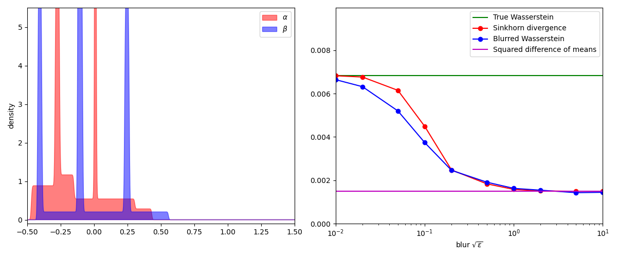
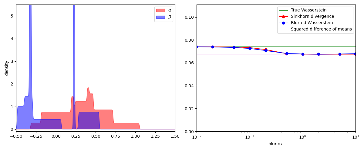
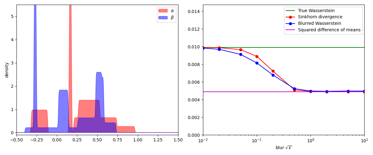
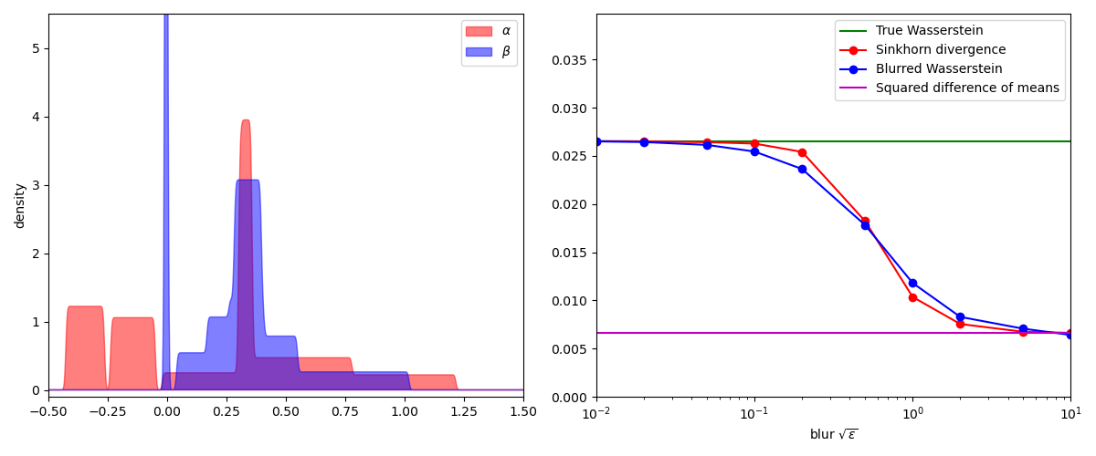
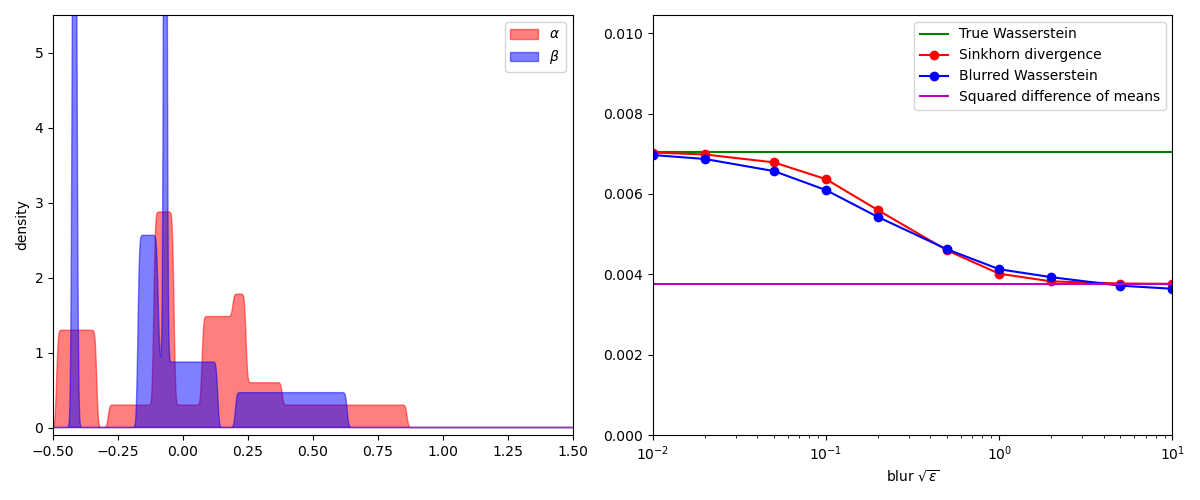
To compare the Sinkhorn and blurred Wasserstein divergences, a simple experiment is to display their values on pairs of 1D measures for increasing values of the temperature \(\varepsilon\): having generated random samples \(\alpha\) and \(\beta\) on the unit interval, we can simply compute \(\text{S}_\varepsilon(\alpha,\beta)\) with our SamplesLoss("sinkhorn") layer while the blurred Wasserstein loss \(\text{B}_\varepsilon(\alpha,\beta)\) can be quickly approximated with the addition of a Gaussian noise followed by a sorting pass.

Setup

Standard imports:

import numpy as np
import matplotlib.pyplot as plt
from sklearn.neighbors import KernelDensity  # display as density curves

import torch
from geomloss import SamplesLoss

use_cuda = torch.cuda.is_available()
#  N.B.: We use float64 numbers to get nice limits when blur -> +infinity
dtype = torch.cuda.DoubleTensor if use_cuda else torch.DoubleTensor

Display routine:

t_plot = np.linspace(-0.5, 1.5, 1000)[:, np.newaxis]


def display_samples(ax, x, color, label=None):
    """Displays samples on the unit interval using a density curve."""
    kde = KernelDensity(kernel="gaussian", bandwidth=0.005).fit(x.data.cpu().numpy())
    dens = np.exp(kde.score_samples(t_plot))
    dens[0] = 0
    dens[-1] = 0
    ax.fill(t_plot, dens, color=color, label=label)

Experiment

def rweight():
    """Random weight."""
    return torch.rand(1).type(dtype)


N = 100 if not use_cuda else 10 ** 3  # Number of samples per measure
C = 100 if not use_cuda else 10000  # number of copies for the Gaussian blur

for _ in range(5):  # Repeat the experiment 5 times
    K = 5  # Generate random 1D measures as the superposition of K=5 intervals
    t = torch.linspace(0, 1, N // K).type(dtype).view(-1, 1)
    X_i = torch.cat([rweight() ** 2 * t + rweight() - 0.5 for k in range(K)], dim=0)
    Y_j = torch.cat([rweight() ** 2 * t + rweight() - 0.5 for k in range(K)], dim=0)

    # Compute the limits when blur = 0...
    x_, _ = X_i.sort(dim=0)
    y_, _ = Y_j.sort(dim=0)
    true_wass = (0.5 / len(X_i)) * ((x_ - y_) ** 2).sum()
    true_wass = true_wass.item()
    # and when blur = +infinity:
    mean_diff = 0.5 * ((X_i.mean(0) - Y_j.mean(0)) ** 2).sum()
    mean_diff = mean_diff.item()

    blurs = [0.01, 0.02, 0.05, 0.1, 0.2, 0.5, 1.0, 2.0, 5.0, 10.0]
    sink, bwass = [], []

    for blur in blurs:
        # Compute the Sinkhorn divergence:
        # N.B.: To be super-precise, we use the well-tested "online" backend
        #       with a very large 'scaling' coefficient
        loss = SamplesLoss("sinkhorn", p=2, blur=blur, scaling=0.99, backend="online")
        sink.append(loss(X_i, Y_j).item())

        # Compute the blurred Wasserstein distance:
        x_i = torch.cat([X_i] * C, dim=0)
        y_j = torch.cat([Y_j] * C, dim=0)
        x_i = x_i + 0.5 * blur * torch.randn(x_i.shape).type(dtype)
        y_j = y_j + 0.5 * blur * torch.randn(y_j.shape).type(dtype)
        x_, _ = x_i.sort(dim=0)
        y_, _ = y_j.sort(dim=0)

        wass = (0.5 / len(x_i)) * ((x_ - y_) ** 2).sum()
        bwass.append(wass.item())

    # Fancy display:
    plt.figure(figsize=(12, 5))

    if N < 10 ** 5:
        ax = plt.subplot(1, 2, 1)
        display_samples(ax, X_i, (1.0, 0, 0, 0.5), label="$\\alpha$")
        display_samples(ax, Y_j, (0, 0, 1.0, 0.5), label="$\\beta$")
        plt.axis([-0.5, 1.5, -0.1, 5.5])
        plt.ylabel("density")
        ax.legend()
        plt.tight_layout()

    ax = plt.subplot(1, 2, 2)
    plt.plot([0.01, 10], [true_wass, true_wass], "g", label="True Wasserstein")
    plt.plot(blurs, sink, "r-o", label="Sinkhorn divergence")
    plt.plot(blurs, bwass, "b-o", label="Blurred Wasserstein")
    plt.plot(
        [0.01, 10], [mean_diff, mean_diff], "m", label="Squared difference of means"
    )
    ax.set_xscale("log")
    ax.legend()
    plt.axis([0.01, 10.0, 0.0, 1.5 * bwass[0]])
    plt.xlabel("blur $\\sqrt{\\varepsilon}$")
    plt.tight_layout()
    plt.show()

• 
• 
• 
• 
• 

Conclusion

In practice, the Sinkhorn and blurred Wasserstein divergences are nearly indistinguishable. But as far as we can tell today, these two loss functions have very different properties:

• \(\text{B}_\varepsilon\) is easy to define, compute in 1D and analyze from geometric or statistical point of views… But cannot (?) be computed efficiently in higher dimensions, where the true OT problem is nearly intractable.

• \(\text{S}_\varepsilon\) is simply available through the SamplesLoss("sinkhorn") layer, but has a weird, composite definition and is pretty hard to study rigorously - as evidenced by recent, technical proofs of positivity, definiteness (Feydy et al., 2018) and sample complexity (Genevay et al., 2018).

So couldn’t we get the best of both worlds? In an ideal world, we’d like to tweak the efficient multiscale Sinkhorn algorithm to compute the natural divergence \(\text{B}_\varepsilon\)… but this may be out of reach. A realistic target could be to quantify the difference between these two objects, thus legitimizing the use of the SamplesLoss("sinkhorn") layer as a cheap proxy for the intuitive and well-understood blurred Wasserstein distance.

In my opinion, investigating the link between these two quantities is one of the most interesting questions left open in the field of discrete entropic OT. The geometric loss functions implemented in GeomLoss are probably good enough for most practical purposes, but getting a rigorous understanding of the multiscale, wavelet-like behavior of our algorithms as we add small details through an exponential decay of the blurring scale \(\sqrt{\varepsilon}\) would be truly insightful. In some sense, couldn’t we prove a Hilbert-Plancherel theorem for the Wasserstein distance?