Sum reduction

Let’s compute the (3000,3) tensor \(c\) whose entries \(c_i^u\) are given by:

\[c_i^u = \sum_j (p-a_j)^2 \exp(x_i^u+y_j^u)\]

where

• \(x\) is a (3000,3) tensor, with entries \(x_i^u\).

• \(y\) is a (5000,3) tensor, with entries \(y_j^u\).

• \(a\) is a (5000,1) tensor, with entries \(a_j\).

• \(p\) is a scalar, encoded as a vector of size (1,).

Setup

Standard imports:

import matplotlib.pyplot as plt
import numpy as np

from pykeops.numpy import Genred

Declare random inputs:

M = 30
N = 50

dtype = "float32"  # May be 'float32' or 'float64'

x = np.random.randn(M, 3).astype(dtype)
y = np.random.randn(N, 3).astype(dtype)
a = np.random.randn(N, 1).astype(dtype)
p = np.random.randn(1).astype(dtype)

Define a custom formula

formula = "Square(p-a)*Exp(x+y)"
variables = [
    "x = Vi(3)",  # First arg   : i-variable, of size 3
    "y = Vj(3)",  # Second arg  : j-variable, of size 3
    "a = Vj(1)",  # Third arg   : j-variable, of size 1 (scalar)
    "p = Pm(1)",
]  # Fourth  arg : Parameter,  of size 1 (scalar)

Our sum reduction is performed over the index \(j\), i.e. on the axis 1 of the kernel matrix. The output c is an \(x\)-variable indexed by \(i\).

my_routine = Genred(formula, variables, reduction_op="Sum", axis=1)
c = my_routine(x, y, a, p, backend="auto")

The equivalent code in NumPy:

c_np = (
    (
        (p - a.T)[:, np.newaxis] ** 2
        * np.exp(x.T[:, :, np.newaxis] + y.T[:, np.newaxis, :])
    )
    .sum(2)
    .T
)

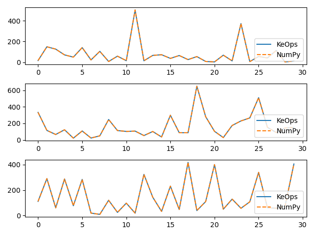
# Plot the results next to each other:
for i in range(3):
    plt.subplot(3, 1, i + 1)
    plt.plot(c[:40, i], "-", label="KeOps")
    plt.plot(c_np[:40, i], "--", label="NumPy")
    plt.legend(loc="lower right")
plt.tight_layout()
plt.show()

Compute the gradient

Now, let’s compute the gradient of \(c\) with respect to \(y\). Since \(c\) is not scalar valued, its “gradient” \(\partial c\) should be understood as the adjoint of the differential operator, i.e. as the linear operator that:

• takes as input a new tensor \(e\) with the shape of \(c\)

• outputs a tensor \(g\) with the shape of \(y\)

such that for all variation \(\delta y\) of \(y\) we have:

\[\langle \text{d} c . \delta y , e \rangle = \langle g , \delta y \rangle = \langle \delta y , \partial c . e \rangle\]

Backpropagation is all about computing the tensor \(g=\partial c . e\) efficiently, for arbitrary values of \(e\):

# Declare a new tensor of shape (M,3) used as the input of the gradient operator.
# It can be understood as a "gradient with respect to the output c"
# and is thus called "grad_output" in the documentation of PyTorch.
e = np.random.randn(M, 3).astype(dtype)

KeOps provides an autodiff engine for formulas. Unfortunately though, as NumPy does not provide any support for backpropagation, we need to specify some informations by hand and add the gradient operator around the formula: Grad(formula , variable_to_differentiate, input_of_the_gradient)

formula_grad = "Grad(" + formula + ", y, e)"

# This new formula makes use of a new variable (the input tensor e)
variables_grad = variables + [
    "e = Vi(3)"
]  # Fifth arg: an i-variable of size 3... Just like "c"!

# The summation is done with respect to the 'i' index (axis=0) in order to get a 'j'-variable
my_grad = Genred(formula_grad, variables_grad, reduction_op="Sum", axis=0)

g = my_grad(x, y, a, p, e)

To generate an equivalent code in numpy, we must compute explicitly the adjoint of the differential (a.k.a. the derivative). To do so, let see \(c^i_u\) as a function of \(y_j\):

\[g_j^u = [(\partial_{y} c^u(y)) . e^u]_j = \sum_{i} (p-a_j)^2 \exp(x_i^u+y_j^u) \cdot e_i^u\]

and implement the formula:

g_np = (
    (
        (p - a.T)[:, np.newaxis, :] ** 2
        * np.exp(x.T[:, :, np.newaxis] + y.T[:, np.newaxis, :])
        * e.T[:, :, np.newaxis]
    )
    .sum(1)
    .T
)

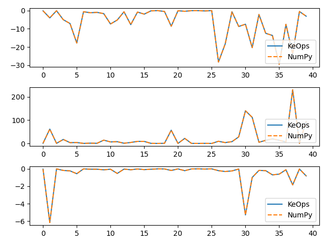
# Plot the results next to each other:
for i in range(3):
    plt.subplot(3, 1, i + 1)
    plt.plot(g[:40, i], "-", label="KeOps")
    plt.plot(g_np[:40, i], "--", label="NumPy")
    plt.legend(loc="lower right")
plt.tight_layout()
plt.show()