Kernel interpolation - PyTorch API

The pykeops.torch.LazyTensor.solve(b, alpha=1e-10) method of KeOps pykeops.torch.LazyTensor allows you to solve optimization problems of the form

\[a^{\star}=\operatorname*{argmin}_a \| (\alpha\operatorname{Id}+K_{xx})a -b\|^2_2,\]

where \(K_{xx}\) is a symmetric, positive definite linear operator defined through the KeOps generic syntax and \(\alpha\) is a nonnegative regularization parameter. In the following script, we use it to solve large-scale Kriging (aka. Gaussian process regression or generalized spline interpolation) problems with a linear memory footprint.

Setup

Standard imports:

import time

import torch
from matplotlib import pyplot as plt

from pykeops.torch import LazyTensor

Generate some data:

use_cuda = torch.cuda.is_available()
dtype = torch.cuda.FloatTensor if use_cuda else torch.FloatTensor

N = 10000 if use_cuda else 1000  # Number of samples

# Sampling locations:
x = torch.rand(N, 1).type(dtype)

# Some random-ish 1D signal:
b = (
    x
    + 0.5 * (6 * x).sin()
    + 0.1 * (20 * x).sin()
    + 0.05 * torch.randn(N, 1).type(dtype)
)

Interpolation in 1D

Specify our regression model - a simple Gaussian variogram or kernel matrix of deviation sigma:

def gaussian_kernel(x, y, sigma=0.1):
    x_i = LazyTensor(x[:, None, :])  # (M, 1, 1)
    y_j = LazyTensor(y[None, :, :])  # (1, N, 1)
    D_ij = ((x_i - y_j) ** 2).sum(-1)  # (M, N) symbolic matrix of squared distances
    return (-D_ij / (2 * sigma**2)).exp()  # (M, N) symbolic Gaussian kernel matrix

Perform the Kernel interpolation, without forgetting to specify the ridge regularization parameter alpha which controls the trade-off between a perfect fit (alpha = 0) and a smooth interpolation (alpha = \(+\infty\)):

alpha = 1.0  # Ridge regularization

start = time.time()

K_xx = gaussian_kernel(x, x)
a = K_xx.solve(b, alpha=alpha)

end = time.time()

print(
    "Time to perform an RBF interpolation with {:,} samples in 1D: {:.5f}s".format(
        N, end - start
    )
)

Time to perform an RBF interpolation with 10,000 samples in 1D: 0.01997s

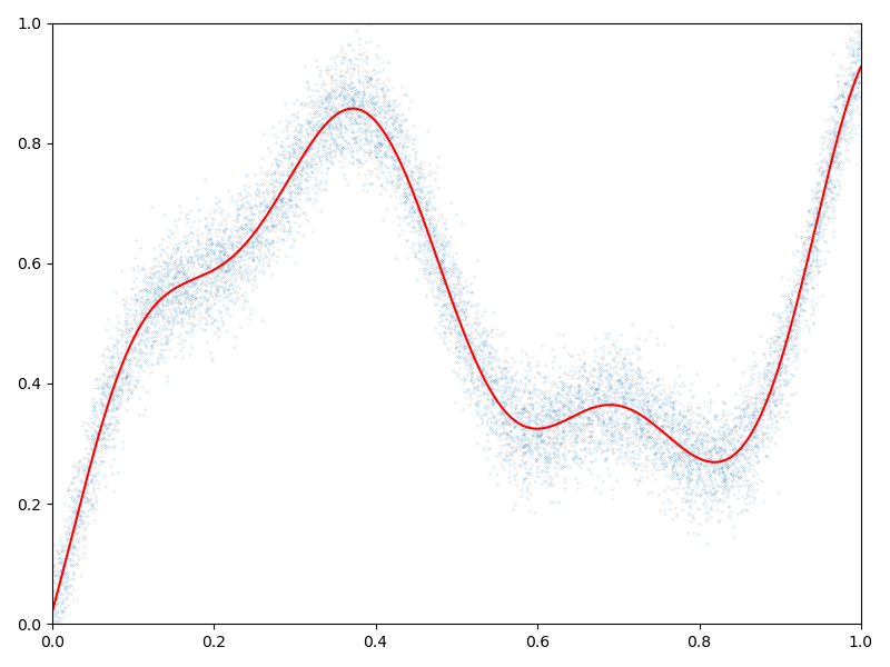
Display the (fitted) model on the unit interval:

# Extrapolate on a uniform sample:
t = torch.linspace(0, 1, 1001).type(dtype)[:, None]

K_tx = gaussian_kernel(t, x)
mean_t = K_tx @ a

# 1D plot:
plt.figure(figsize=(8, 6))

plt.scatter(x.cpu()[:, 0], b.cpu()[:, 0], s=100 / len(x))  # Noisy samples
plt.plot(t.cpu().numpy(), mean_t.cpu().numpy(), "r")

plt.axis([0, 1, 0, 1])
plt.tight_layout()

Interpolation in 2D

Generate some data:

# Sampling locations:
x = torch.rand(N, 2).type(dtype)

# Some random-ish 2D signal:
b = ((x - 0.5) ** 2).sum(1, keepdim=True)
b[b > 0.4**2] = 0
b[b < 0.3**2] = 0
b[b >= 0.3**2] = 1
b = b + 0.05 * torch.randn(N, 1).type(dtype)

# Add 25% of outliers:
Nout = N // 4
b[-Nout:] = torch.rand(Nout, 1).type(dtype)

Specify our regression model - a simple Exponential variogram or Laplacian kernel matrix of deviation sigma:

def laplacian_kernel(x, y, sigma=0.1):
    x_i = LazyTensor(x[:, None, :])  # (M, 1, 1)
    y_j = LazyTensor(y[None, :, :])  # (1, N, 1)
    D_ij = ((x_i - y_j) ** 2).sum(-1)  # (M, N) symbolic matrix of squared distances
    return (-D_ij.sqrt() / sigma).exp()  # (M, N) symbolic Laplacian kernel matrix

Perform the Kernel interpolation, without forgetting to specify the ridge regularization parameter alpha which controls the trade-off between a perfect fit (alpha = 0) and a smooth interpolation (alpha = \(+\infty\)):

alpha = 10  # Ridge regularization

start = time.time()

K_xx = laplacian_kernel(x, x)
a = K_xx.solve(b, alpha=alpha)

end = time.time()

print(
    "Time to perform an RBF interpolation with {:,} samples in 2D: {:.5f}s".format(
        N, end - start
    )
)

Time to perform an RBF interpolation with 10,000 samples in 2D: 0.02437s

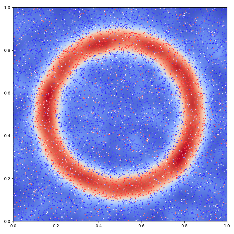
Display the (fitted) model on the unit square:

# Extrapolate on a uniform sample:
X = Y = torch.linspace(0, 1, 101).type(dtype)
X, Y = torch.meshgrid(X, Y)
t = torch.stack((X.contiguous().view(-1), Y.contiguous().view(-1)), dim=1)

K_tx = laplacian_kernel(t, x)
mean_t = K_tx @ a
mean_t = mean_t.view(101, 101)

# 2D plot: noisy samples and interpolation in the background
plt.figure(figsize=(8, 8))

plt.scatter(
    x.cpu()[:, 0], x.cpu()[:, 1], c=b.cpu().view(-1), s=25000 / len(x), cmap="bwr"
)
plt.imshow(
    mean_t.cpu().numpy()[::-1, :],
    interpolation="bilinear",
    extent=[0, 1, 0, 1],
    cmap="coolwarm",
)

# sphinx_gallery_thumbnail_number = 2
plt.axis([0, 1, 0, 1])
plt.tight_layout()
plt.show()

/opt/conda/lib/python3.11/site-packages/torch/functional.py:507: UserWarning: torch.meshgrid: in an upcoming release, it will be required to pass the indexing argument. (Triggered internally at /opt/conda/conda-bld/pytorch_1704987288773/work/aten/src/ATen/native/TensorShape.cpp:3549.)
  return _VF.meshgrid(tensors, **kwargs)  # type: ignore[attr-defined]