Unstructured Shape Matching

In this tutorial, we register two curves with IMODAL without deformation prior. To achieve this, a local translation deformation module is used.

Initialization

Import relevant Python modules.

import sys
sys.path.append("../")

import math
import copy

import torch
import matplotlib.pyplot as plt

import imodal

imodal.Utilities.set_compute_backend('torch')

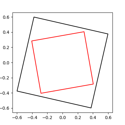
First, we generate the source (circle) and the target (square) and plot them.

nb_points_square_side = 12
source = imodal.Utilities.generate_unit_square(nb_points_square_side)
source = imodal.Utilities.linear_transform(source, imodal.Utilities.rot2d(-math.pi/14.))


nb_points_square_side = 4
target = 0.7*imodal.Utilities.generate_unit_square(nb_points_square_side)
target = imodal.Utilities.linear_transform(target, imodal.Utilities.rot2d(math.pi/18.))


plt.figure(figsize=[4., 4.])

imodal.Utilities.plot_closed_shape(source, color='black')
imodal.Utilities.plot_closed_shape(target, color='red')

plt.axis('equal')

plt.subplots_adjust(left=0.1, right=0.9, top=0.9, bottom=0.1)
plt.show()

From these objects, DeformablePoints are created to be used for the registration. This is a sub class of Deformables which represents geometrical objects that can be deformed by the framework.

source_deformable = imodal.Models.DeformablePoints(source)
target_deformable = imodal.Models.DeformablePoints(target)

We define the local translation module translation: we need to specify the gaussian kernel scale (sigma_translation). We initialize its geometrical descriptor (gd) with the source points.

sigma_translation = 1.
translation = imodal.DeformationModules.ImplicitModule0(2, source.shape[0], sigma_translation, nu=1e-4, gd=source)

The distance between the deformed source and the target is measured using the varifold framework, which does not require point correspondance. The spatial kernel is a scalar gaussian kernel for which we specify the scale sigma_varifold.

sigma_varifold = [0.5]
attachment = imodal.Attachment.VarifoldAttachment(2, sigma_varifold, backend='torch')

Registration

We create the registration model. The lam parameter is the weight of the attachment term of the total energy to minimize.

model = imodal.Models.RegistrationModel(source_deformable, [translation], attachment, lam=100.)

We launch the energy minimization using the Fitter class. We specify the ODE solver algorithm shoot_solver and the number of iteration steps shoot_it used to integrate the shooting equation. The optimizer can be manually selected. Here, we select Pytorch’s LBFGS algorithm with strong Wolfe termination conditions. max_iter defines the maximum number of iteration for the optimization.

shoot_solver = 'euler'
shoot_it = 10

fitter = imodal.Models.Fitter(model, optimizer='torch_lbfgs')
max_iter = 10

fitter.fit(target_deformable, max_iter, options={'line_search_fn': 'strong_wolfe', 'shoot_solver': shoot_solver, 'shoot_it': shoot_it})

Out:

Starting optimization with method torch LBFGS, using solver euler with 10 iterations.
Initial cost={'deformation': 0.0, 'attach': 54.57539367675781}
1e-10
Evaluated model with costs=54.57539367675781
Evaluated model with costs=19.14338093996048
Evaluated model with costs=6.4000039249658585
Evaluated model with costs=3.1447209417819977
Evaluated model with costs=1.5842044353485107
Evaluated model with costs=9.115530669689178
Evaluated model with costs=1.26090669631958
Evaluated model with costs=0.8082702159881592
Evaluated model with costs=0.602929562330246
Evaluated model with costs=0.4900495111942291
Evaluated model with costs=0.479810893535614
Evaluated model with costs=0.48361146450042725
Evaluated model with costs=0.4796399474143982
Evaluated model with costs=0.47953301668167114
Evaluated model with costs=0.47956109046936035
Evaluated model with costs=0.4795800745487213
Evaluated model with costs=0.4795333743095398
Evaluated model with costs=0.4795810580253601
================================================================================
Time: 2.8076504664495587
Iteration: 0
Costs
deformation=0.3482601046562195
attach=0.13132095336914062
Total cost=0.4795810580253601
1e-10
Evaluated model with costs=0.47953301668167114
Evaluated model with costs=0.47956109046936035
Evaluated model with costs=0.4795800745487213
Evaluated model with costs=0.4795333743095398
Evaluated model with costs=0.4795810580253601
================================================================================
Time: 3.6211067866533995
Iteration: 1
Costs
deformation=0.3482601046562195
attach=0.13132095336914062
Total cost=0.4795810580253601
================================================================================
Optimisation process exited with message: Convergence achieved.
Final cost=0.4795810580253601
Model evaluation count=23
Time elapsed = 3.6212978567928076

Displaying results

We compute the optimized deformation.

intermediates = {}
with torch.autograd.no_grad():
    deformed = model.compute_deformed(shoot_solver, shoot_it, intermediates=intermediates)[0][0]

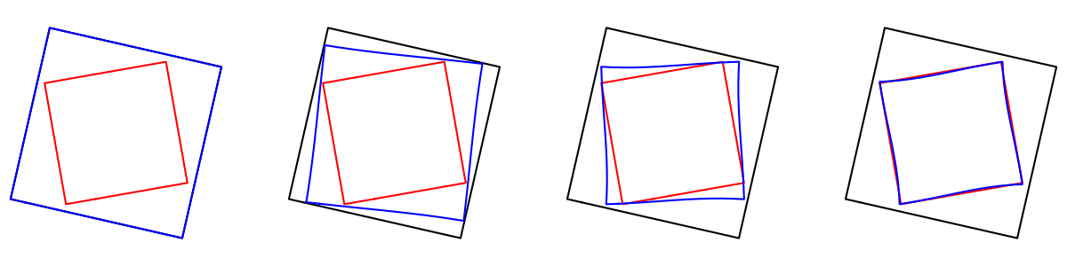
We display the result.

display_index = [0, 3, 7, 10]
plt.figure(figsize=[3.*len(display_index), 3.])
for count, i in enumerate(display_index):
    plt.subplot(1, len(display_index), 1+count).set_title("t={}".format(i/10.))
    deformed_i = intermediates['states'][i][0].gd
    imodal.Utilities.plot_closed_shape(source, color='black')
    imodal.Utilities.plot_closed_shape(target, color='red')
    imodal.Utilities.plot_closed_shape(deformed_i, color='blue')
    plt.axis('equal')
    plt.axis('off')
plt.subplots_adjust(left=0., right=1., top=1., bottom=0.)
plt.show()

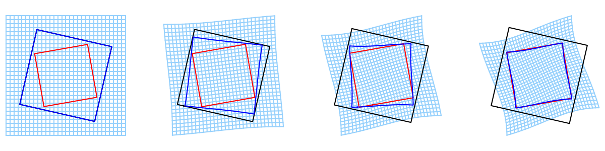
In order to visualize the deformation, we will compute the grid deformation. We first retrieve the modules and initialize their manifolds (with initial values of geometrical descriptor and momentum).

modules = imodal.DeformationModules.CompoundModule(copy.copy(model.modules))
modules.manifold.fill(model.init_manifold.clone())

We initialize a grid built from a bounding box and a grid resolution. We create a bounding box aabb around the source, scaled with a 1.3 factor to enhance the visualization of the deformation. Then, we define the grid resolution grid_resolution from the size of each grid gap square_size. Finally, we create a silent deformation module deformation_grid whose geometrical descriptor is made of the grid points.

aabb = imodal.Utilities.AABB.build_from_points(source).scale(1.3)
square_size = 0.05
grid_resolution = [math.floor(aabb.width/square_size),
                   math.floor(aabb.height/square_size)]

deformation_grid = imodal.DeformationModules.DeformationGrid(aabb, grid_resolution)

We inject the newly created deformation module deformation_grid into the list of deformation modules modules_grid. We create the hamiltonian structure hamiltonian allowing us to integrate the shooting equation. We then recompute the deformation, now tracking the grid deformation.

modules_grid = [*modules, deformation_grid]
hamiltonian = imodal.HamiltonianDynamic.Hamiltonian(modules_grid)

intermediates_grid = {}
with torch.autograd.no_grad():
    imodal.HamiltonianDynamic.shoot(hamiltonian, shoot_solver, shoot_it, intermediates=intermediates_grid)

We display the result along with the deformation grid.

display_index = [0, 3, 7, 10]
plt.figure(figsize=[3.*len(display_index), 3.])
for count, i in enumerate(display_index):
    ax = plt.subplot(1, len(display_index), 1+count)
    deformed_i = intermediates_grid['states'][i][0].gd
    deformation_grid.manifold.fill_gd(intermediates_grid['states'][i][-1].gd)
    grid_x, grid_y = deformation_grid.togrid()
    imodal.Utilities.plot_grid(ax, grid_x, grid_y, color='xkcd:light blue')
    imodal.Utilities.plot_closed_shape(source, color='black')
    imodal.Utilities.plot_closed_shape(target, color='red')
    imodal.Utilities.plot_closed_shape(deformed_i, color='blue')
    plt.axis('equal')
    plt.axis('off')
plt.subplots_adjust(left=0., right=1., top=1., bottom=0.)
plt.show()