Fitting a Gaussian Mixture Model

In this tutorial, we show how to use KeOps to fit a Gaussian Mixture Model with a custom sparsity prior through gradient descent on the empiric log-likelihood.

Setup

Standard imports:

import matplotlib.cm as cm
import numpy as np
import torch
from matplotlib import pyplot as plt
from torch.nn import Module
from torch.nn.functional import softmax, log_softmax

from pykeops.torch import Vi, Vj, LazyTensor

Define our dataset: a collection of points $(x_{i})_{i \in [1, N]}$ which describe a spiral in the unit square.

# Choose the storage place for our data : CPU (host) or GPU (device) memory.
dtype = torch.cuda.FloatTensor if torch.cuda.is_available() else torch.FloatTensor
torch.manual_seed(0)
N = 10000  # Number of samples
t = torch.linspace(0, 2 * np.pi, N + 1)[:-1]
x = torch.stack((0.5 + 0.4 * (t / 7) * t.cos(), 0.5 + 0.3 * t.sin()), 1)
x = x + 0.02 * torch.randn(x.shape)
x = x.type(dtype)
x.requires_grad = True

Display:

# Create a uniform grid on the unit square:
res = 200
ticks = np.linspace(0, 1, res + 1)[:-1] + 0.5 / res
X, Y = np.meshgrid(ticks, ticks)

grid = torch.from_numpy(np.vstack((X.ravel(), Y.ravel())).T).contiguous().type(dtype)

Gaussian Mixture Model

In this tutorial, we focus on a Gaussian Mixture Model with varying covariance matrices. For all class indices $j$ in $[1, M]$ , we denote by $w_{j}$ the weight score of the $j$ -th class, i.e. the real number such that

W_{j} = \frac{\exp (w_{j})}{\sum_{k} \exp (w_{k})}

is the probability assigned to the $j$ -th component of the mixture. Then, we encode the (inverse) covariance matrix $Σ_{j}^{- 1}$ of this component through an arbitrary matrix $A_{j}$ :

Σ_{j}^{- 1} = A_{j} A_{j}^{⊺}

and can evaluate the likelihood of our model at any point $x$ through:

{likelihood}_{(w_{j}), (A_{j})} (x) = \sum_{j = 1}^{M} W_{j} \cdot (2 π)^{- D / 2} \cdot \sqrt{det (A_{j} A_{j}^{⊺})} \cdot e^{- \frac{1}{2} (x - μ_{j})^{⊺} A_{j} A_{j}^{⊺} (x - μ_{j})} .

The log-likelihood of a sample $(x_{i})$ with respect to the parameters $(A_{j})$ and $(w_{j})$ can thus be computed using a straightforward log-sum-exp reduction, which is most easily implemented through the pykeops.torch.LazyTensor() interface.

Custom sparsity prior. Going further, we may allow our model to select adaptively the number of active components by adding a sparsity-inducing penalty on the class weights $W_{j}$ . For instance, we could minimize the cost:

{Cost}_{(x_{i})} ((w_{j}), (A_{j})) = - \frac{1}{N} \sum_{i = 1}^{N} \log {likelihood}_{(w_{j}), (A_{j})} (x_{i}) + \frac{s}{M} \sum_{j = 1}^{M} \sqrt{W_{j}},

where the sparsity coefficient $s$ controls the amount of non-empty clusters. Even though this energy cannot be optimized in closed form through an EM-like algorithm, automatic differentiation allows us to fit this custom model without hassle:

class GaussianMixture(Module):
    def __init__(self, M, sparsity=0, D=2):
        super(GaussianMixture, self).__init__()

        self.params = {}
        # We initialize our model with random blobs scattered across
        # the unit square, with a small-ish radius:
        self.mu = torch.rand(M, D).type(dtype)
        self.A = 15 * torch.ones(M, 1, 1) * torch.eye(D, D).view(1, D, D)
        self.A = (self.A).type(dtype).contiguous()
        self.w = torch.ones(M, 1).type(dtype)
        self.sparsity = sparsity
        self.mu.requires_grad, self.A.requires_grad, self.w.requires_grad = (
            True,
            True,
            True,
        )

    def update_covariances(self):
        """Computes the full covariance matrices from the model's parameters."""
        (M, D, _) = self.A.shape
        self.params["gamma"] = (torch.matmul(self.A, self.A.transpose(1, 2))).view(
            M, D * D
        ) / 2

    def covariances_determinants(self):
        """Computes the determinants of the covariance matrices.

        N.B.: PyTorch still doesn't support batched determinants, so we have to
              implement this formula by hand.
        """
        S = self.params["gamma"]
        if S.shape[1] == 2 * 2:
            dets = S[:, 0] * S[:, 3] - S[:, 1] * S[:, 2]
        else:
            raise NotImplementedError
        return dets.view(-1, 1)

    def weights(self):
        """Scalar factor in front of the exponential, in the density formula."""
        return softmax(self.w, 0) * self.covariances_determinants().sqrt()

    def weights_log(self):
        """Logarithm of the scalar factor, in front of the exponential."""
        return log_softmax(self.w, 0) + 0.5 * self.covariances_determinants().log()

    def likelihoods(self, sample):
        """Samples the density on a given point cloud."""
        self.update_covariances()
        return (
            -Vi(sample).weightedsqdist(Vj(self.mu), Vj(self.params["gamma"]))
        ).exp() @ self.weights()

    def log_likelihoods(self, sample):
        """Log-density, sampled on a given point cloud."""
        self.update_covariances()
        K_ij = -Vi(sample).weightedsqdist(Vj(self.mu), Vj(self.params["gamma"]))
        return K_ij.logsumexp(dim=1, weight=Vj(self.weights()))

    def neglog_likelihood(self, sample):
        """Returns -log(likelihood(sample)) up to an additive factor."""
        ll = self.log_likelihoods(sample)
        log_likelihood = torch.mean(ll)
        # N.B.: We add a custom sparsity prior, which promotes empty clusters
        #       through a soft, concave penalization on the class weights.
        return -log_likelihood + self.sparsity * softmax(self.w, 0).sqrt().mean()

    def get_sample(self, N):
        """Generates a sample of N points."""
        raise NotImplementedError()

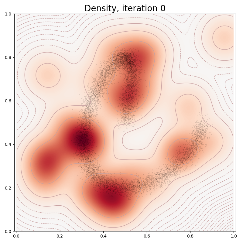
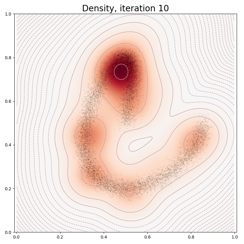
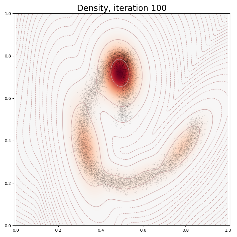
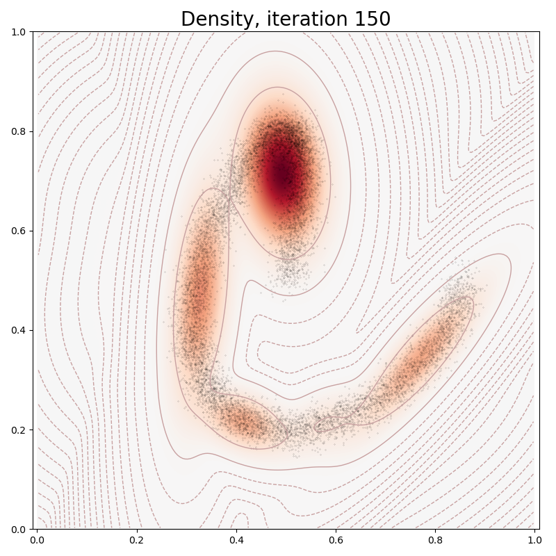
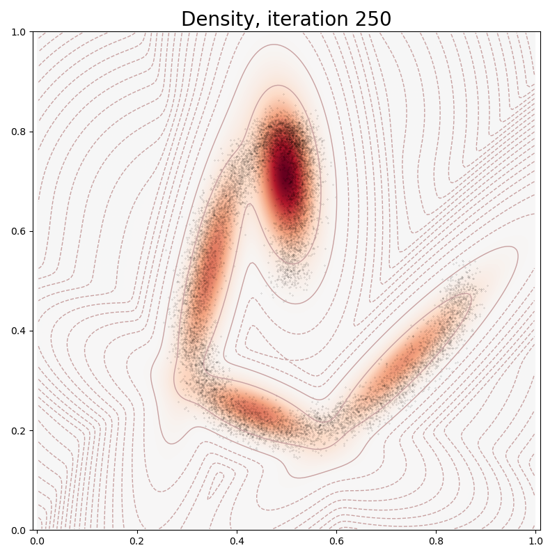
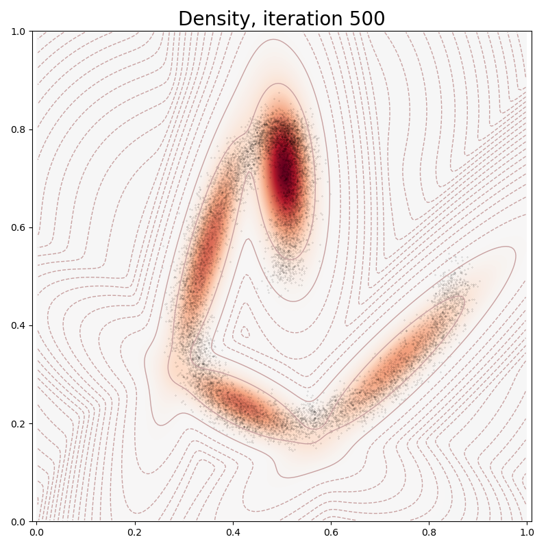
    def plot(self, sample):
        """Displays the model."""
        plt.clf()
        # Heatmap:
        heatmap = self.likelihoods(grid)
        heatmap = (
            heatmap.view(res, res).data.cpu().numpy()
        )  # reshape as a "background" image

        scale = np.amax(np.abs(heatmap[:]))
        plt.imshow(
            -heatmap,
            interpolation="bilinear",
            origin="lower",
            vmin=-scale,
            vmax=scale,
            cmap=cm.RdBu,
            extent=(0, 1, 0, 1),
        )

        # Log-contours:
        log_heatmap = self.log_likelihoods(grid)
        log_heatmap = log_heatmap.view(res, res).data.cpu().numpy()

        scale = np.amax(np.abs(log_heatmap[:]))
        levels = np.linspace(-scale, scale, 41)

        plt.contour(
            log_heatmap,
            origin="lower",
            linewidths=1.0,
            colors="#C8A1A1",
            levels=levels,
            extent=(0, 1, 0, 1),
        )

        # Scatter plot of the dataset:
        xy = sample.data.cpu().numpy()
        plt.scatter(xy[:, 0], xy[:, 1], 100 / len(xy), color="k")

Optimization

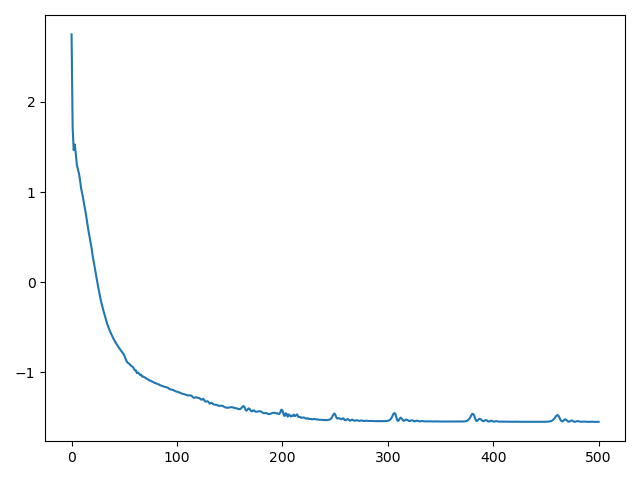
In typical PyTorch fashion, we fit our Mixture Model to the data through a stochastic gradient descent on our empiric log-likelihood, with a sparsity-inducing penalty:

model = GaussianMixture(30, sparsity=20)
optimizer = torch.optim.Adam([model.A, model.w, model.mu], lr=0.1)
loss = np.zeros(501)

for it in range(501):
    optimizer.zero_grad()  # Reset the gradients (PyTorch syntax...).
    cost = model.neglog_likelihood(x)  # Cost to minimize.
    cost.backward()  # Backpropagate to compute the gradient.
    optimizer.step()
    loss[it] = cost.data.cpu().numpy()

    # sphinx_gallery_thumbnail_number = 6
    if it in [0, 10, 100, 150, 250, 500]:
        plt.pause(0.01)
        plt.figure(figsize=(8, 8))
        model.plot(x)
        plt.title("Density, iteration " + str(it), fontsize=20)
        plt.axis("equal")
        plt.axis([0, 1, 0, 1])
        plt.tight_layout()
        plt.pause(0.01)

Monitor the optimization process:

plt.figure()
plt.plot(loss)
plt.tight_layout()
plt.show()

Total running time of the script: (0 minutes 3.792 seconds)

Gallery generated by Sphinx-Gallery