Kernel interpolation - NumPy API

The pykeops.numpy.LazyTensor.solve(b, alpha=1e-10) method of KeOps pykeops.numpy.LazyTensor allows you to solve optimization problems of the form

\[\begin{split}& & a^{\star} & =\operatorname*{argmin}_a \tfrac 1 2 \langle a,( \alpha \operatorname{Id}+K_{xx}) a\rangle - \langle a,b \rangle, \\\\ &\text{i.e.}\quad & a^{\star} & = (\alpha \operatorname{Id} + K_{xx})^{-1} b,\end{split}\]

where \(K_{xx}\) is a symmetric, positive definite linear operator defined through the KeOps generic syntax and \(\alpha\) is a nonnegative regularization parameter. In the following script, we use it to solve large-scale Kriging (aka. Gaussian process regression or generalized spline interpolation) problems with a linear memory footprint.

Setup

Standard imports:

import time

import numpy as np
from matplotlib import pyplot as plt

from pykeops.numpy import LazyTensor
import pykeops.config

Generate some data:

dtype = "float64"

N = 10000 if pykeops.config.gpu_available else 1000  # Number of samples

# Sampling locations:
x = np.random.rand(N, 1).astype(dtype)

# Some random-ish 1D signal:
b = (
    x
    + 0.5 * np.sin(6 * x)
    + 0.1 * np.sin(20 * x)
    + 0.05 * np.random.randn(N, 1).astype(dtype)
)

Interpolation in 1D

Specify our regression model - a simple Gaussian variogram or kernel matrix of deviation sigma:

def gaussian_kernel(x, y, sigma=0.1):
    x_i = LazyTensor(x[:, None, :])  # (M, 1, 1)
    y_j = LazyTensor(y[None, :, :])  # (1, N, 1)
    D_ij = ((x_i - y_j) ** 2).sum(-1)  # (M, N) symbolic matrix of squared distances
    return (-D_ij / (2 * sigma**2)).exp()  # (M, N) symbolic Gaussian kernel matrix

Perform the Kernel interpolation, without forgetting to specify the ridge regularization parameter alpha which controls the trade-off between a perfect fit (alpha = 0) and a smooth interpolation (alpha = \(+\infty\)):

alpha = 1.0  # Ridge regularization

start = time.time()

K_xx = gaussian_kernel(x, x)
a = K_xx.solve(b, alpha=alpha)

end = time.time()

print(
    "Time to perform an RBF interpolation with {:,} samples in 1D: {:.5f}s".format(
        N, end - start
    )
)

Time to perform an RBF interpolation with 10,000 samples in 1D: 0.07726s

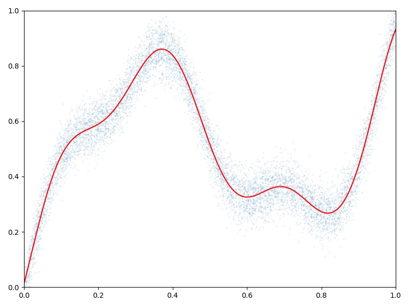
Display the (fitted) model on the unit interval:

# Extrapolate on a uniform sample:
t = np.reshape(np.linspace(0, 1, 1001), [1001, 1]).astype(dtype)

K_tx = gaussian_kernel(t, x)
mean_t = K_tx @ a

# 1D plot:
plt.figure(figsize=(8, 6))

plt.scatter(x[:, 0], b[:, 0], s=100 / len(x))  # Noisy samples
plt.plot(t, mean_t, "r")

plt.axis([0, 1, 0, 1])
plt.tight_layout()

Interpolation in 2D

Generate some data:

# Sampling locations:
x = np.random.rand(N, 2).astype(dtype)

# Some random-ish 2D signal:
b = np.sum((x - 0.5) ** 2, axis=1)[:, None]
b[b > 0.4**2] = 0
b[b < 0.3**2] = 0
b[b >= 0.3**2] = 1
b = b + 0.05 * np.random.randn(N, 1).astype(dtype)

# Add 25% of outliers:
Nout = N // 4
b[-Nout:] = np.random.rand(Nout, 1).astype(dtype)

Specify our regression model - a simple Exponential variogram or Laplacian kernel matrix of deviation sigma:

def laplacian_kernel(x, y, sigma=0.1):
    x_i = LazyTensor(x[:, None, :])  # (M, 1, 1)
    y_j = LazyTensor(y[None, :, :])  # (1, N, 1)
    D_ij = ((x_i - y_j) ** 2).sum(-1)  # (M, N) symbolic matrix of squared distances
    return (-D_ij.sqrt() / sigma).exp()  # (M, N) symbolic Laplacian kernel matrix

Perform the Kernel interpolation, without forgetting to specify the ridge regularization parameter alpha which controls the trade-off between a perfect fit (alpha = 0) and a smooth interpolation (alpha = \(+\infty\)):

alpha = 10  # Ridge regularization

start = time.time()

K_xx = laplacian_kernel(x, x)
a = K_xx.solve(b, alpha=alpha)

end = time.time()

print(
    "Time to perform an RBF interpolation with {:,} samples in 2D: {:.5f}s".format(
        N, end - start
    )
)

Time to perform an RBF interpolation with 10,000 samples in 2D: 0.10685s

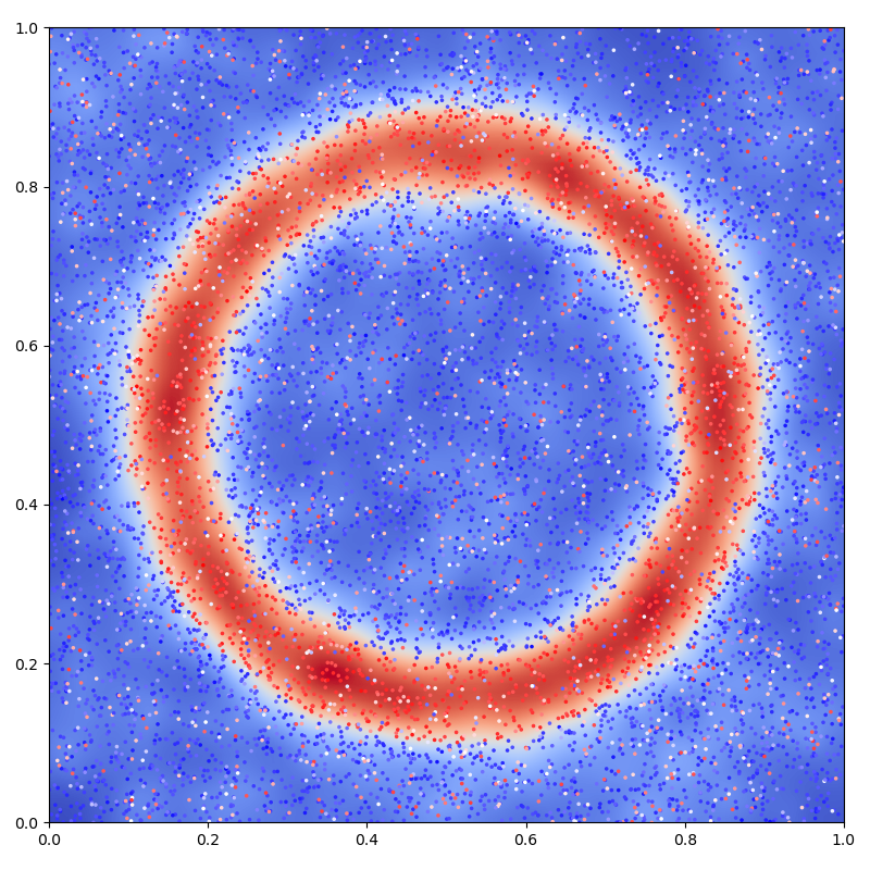
Display the (fitted) model on the unit square:

# Extrapolate on a uniform sample:
X = Y = np.linspace(0, 1, 101)
X, Y = np.meshgrid(X, Y)
t = np.stack((X.ravel(), Y.ravel()), axis=1)

K_tx = laplacian_kernel(t, x)
mean_t = K_tx @ a
mean_t = mean_t.reshape(101, 101)[::-1, :]

# 2D plot: noisy samples and interpolation in the background
plt.figure(figsize=(8, 8))

plt.scatter(x[:, 0], x[:, 1], c=b.ravel(), s=25000 / len(x), cmap="bwr")
plt.imshow(mean_t, interpolation="bilinear", extent=[0, 1, 0, 1], cmap="coolwarm")

plt.axis([0, 1, 0, 1])
plt.tight_layout()
plt.show()