Block-sparsity

Complexity of the KeOps routines. Notwithstanding their finely grained management of memory, the GPU_1D and GPU_2D schemes have a quadratic time complexity: if \(\mathrm{M}\) and \(\mathrm{N}\) denote the number of \(i\) and \(j\) variables, the time needed to perform a generic reduction scales asymptotically in \(O(\mathrm{M}\mathrm{N})\). This is most evident in our convolution benchmarks, where all the kernel coefficients

\[\begin{aligned} K_{ij} ~=~ k(x_i,y_j) ~=~ \exp(-\|x_i-y_j\|^2\,/\,2\sigma^2)\end{aligned}\]

are computed to implement a discrete Gaussian convolution:

\[\begin{aligned} (a_i)~=~ (K_{ij}) \cdot (b_i) \qquad\text{i.e.}\qquad a_i ~=~ \sum_{j=1}^\mathrm{N} k(x_i,y_j)\cdot b_j \qquad \text{for $i\in\left[\!\left[ 1,\mathrm{M} \right]\!\right] $.} \end{aligned}\]

Can we do better?

To break through this quadratic lower bound, a simple idea is to skip some computations, using a sparsity prior on the kernel matrix. For instance, we could decide to skip kernel computations when points \(x_i\) and \(y_j\) are far away from each other. But can we do so efficiently?

Sparsity on the CPU. On CPUs, a standard strategy is to use sparse matrices, encoding our operators through lists of non-zero coefficients and indices. Schematically, this comes down to endowing each index \(i\in\left[\!\left[ 1,\mathrm{M}\right]\!\right]\) with a set \(J_i\subset\left[\!\left[ 1,\mathrm{N}\right]\!\right]\) of \(j\)-neighbors and to restrict ourselves to the computation of

\[\begin{aligned} a_i ~=~ \sum_{j\in J_i} k(x_i,y_j)\cdot b_j, \qquad \text{for $i\in\left[\!\left[ 1,\mathrm{M}\right]\!\right]$.}\end{aligned}\]

This approach is very well suited to matrices which only have a handful of nonzero coefficients per line, such as the intrinsic Laplacian of a 3D mesh. But on large, densely connected problems, sparse encoding runs into a major issue: since it relies on non-contiguous memory accesses, it scales poorly on GPUs.

Block-sparse reductions

As explained in our introduction, GPU chips are wired to rely on coalesced memory operations which load blocks of dozens of contiguous bytes at once. Instead of allowing the use of arbitrary indexing sets \(J_i\) for all lines of our sparse kernel matrix, we should thus restrict ourselves to computations of the form:

\[\begin{aligned} a_i ~=~ \sum_{l=1}^{S_q} \sum_{j=\text{start}^q_l}^{\text{end}^q_l-1} k(x_i,y_j)\cdot b_j, \qquad \text{for $i \in \left[\!\left[\text{start}_q, \text{end}_q\right[\!\right[$~~ and~~ $q\in \left[\!\left[ 1,\mathrm{Q}\right]\!\right]$,}\end{aligned}\]

where:

1. The \(\left[\!\left[\text{start}_q, \text{end}_q\right[\!\right[\) intervals form a partition of the set of \(i\)-indices  \(\left[\!\left[ 1,\mathrm{M}\right]\!\right]\):

   \[\begin{aligned} \left[\!\left[ 1,\mathrm{M}\right]\!\right] ~=~ \bigsqcup_{q=1}^{\mathrm{Q}} \,\left[\!\left[\text{start}_q, \text{end}_q\right[\!\right[. \end{aligned}\]

2. For every segment \(q\in\left[\!\left[ 1,\mathrm{Q}\right]\!\right]\), the \(S_q\) intervals \([\![\text{start}^q_l, \text{end}^q_l[\![\) encode a set of neighbors as a finite collection of contiguous ranges of indices:

   \[\begin{aligned} \forall~i\in \left[\!\left[\text{start}_q, \text{end}_q\right[\!\right[, ~ J_i~=~ \bigsqcup_{l=1}^{S_q} \,[\![\text{start}^q_l, \text{end}^q_l[\![. \end{aligned}\]

By encoding our sparsity patterns as block-wise binary masks made up of tiles

\[\begin{aligned} T^q_l~=~\left[\!\left[\text{start}_q, \text{end}_q\right[\!\right[ \times [\![\text{start}^q_l, \text{end}^q_l[\![ ~~ \subset ~ \left[\!\left[ 1,\mathrm{M}\right]\!\right]\times\left[\!\left[ 1,\mathrm{N}\right]\!\right]~,\end{aligned}\]

we can leverage coalesced memory operations for maximum efficiency on the GPU. As long as our index ranges are wider than the CUDA blocks, we should get close to optimal performances.

Going further. This scheme can be generalized to generic formulas and reductions. For reductions with respect to the \(i\) axis, we simply have to define transposed tiles

\[\begin{aligned} U^q_l~=~[\![\text{start}^q_l, \text{end}^q_l[\![ \times \left[\!\left[\text{start}_q, \text{end}_q\right[\!\right[ ~~ \subset ~ \left[\!\left[ 1,\mathrm{M}\right]\!\right]\times\left[\!\left[ 1,\mathrm{N}\right]\!\right]\end{aligned}\]

and restrict ourselves to computations of the form:

\[\begin{aligned} b_j ~=~ \sum_{l=1}^{S_q} \sum_{i=\text{start}^q_l}^{\text{end}^q_l-1} k(x_i,y_j)\cdot a_i, \qquad \text{for $j \in \left[\!\left[\text{start}_q, \text{end}_q\right[\!\right[$ and $q\in \left[\!\left[ 1,\mathrm{Q}\right]\!\right]$.}\end{aligned}\]

A decent trade-off

This block-wise approach to sparse reductions may seem a bit too coarse, as some negligible coefficients get computed with little to no impact on the final result… But in practice, the GPU speed-ups on contiguous memory operations more than make up for it: implemented in the GpuConv1D_ranges.cu CUDA file, our block-sparse Map-Reduce scheme is the workhorse of the multiscale Sinkhorn algorithm showcased in the GeomLoss library.

As explained in our documentation, the main user interface for KeOps block-sparse reduction is an optional “.ranges” attribute for LazyTensors which encodes arbitrary block-sparsity masks. In practice, as illustrated in the Figure below, helper routines allow users to specify tiled sparsity patterns from clustered arrays of samples \(x_i\), \(y_j\) and coarse cluster-to-cluster boolean matrices. Implementing Barnes-Hut-like strategies and other approximation rules is thus relatively easy, up to a preliminary sorting pass which ensures that all clusters are stored contiguously in memory.

(a) Point clouds.

(b) Coarse boolean mask.

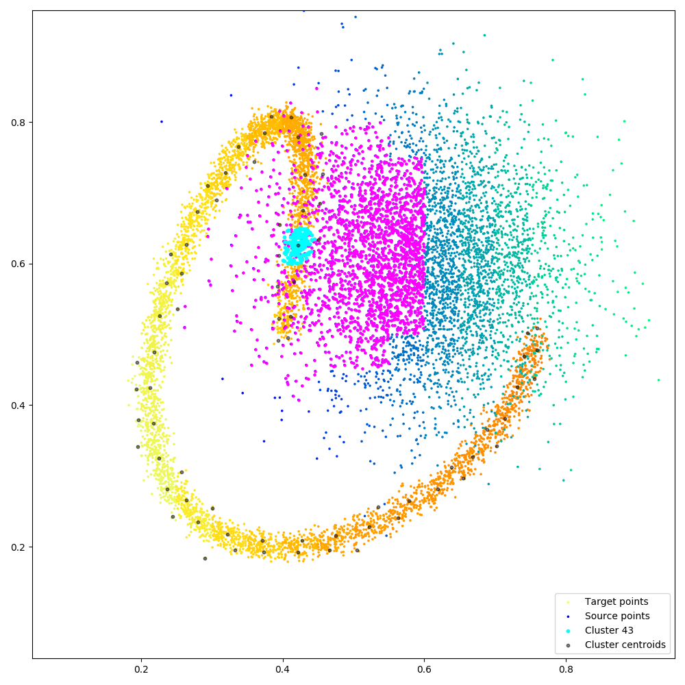
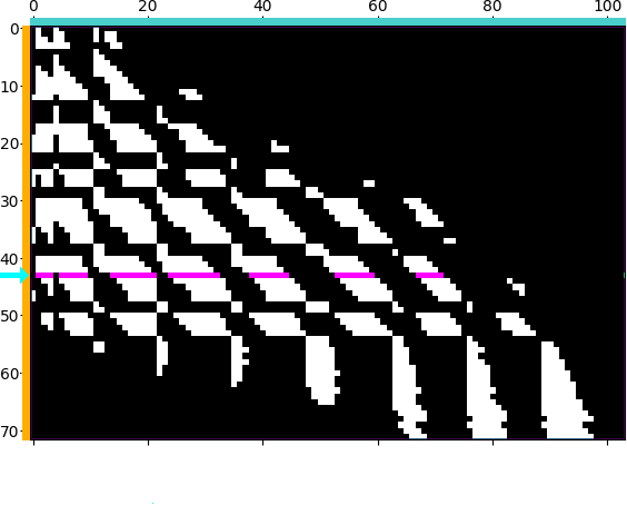
Figure. Illustrating block-sparse reductions with 2D point clouds. When using an \(\mathrm{M}\)-by-\(\mathrm{N}\) “kernel” matrix to compute an interaction term between two datasets, a common approximation strategy is to skip terms which correspond to clusters of points that are far away from each other. Through a set of helper routines and optional arguments, KeOps allows users to implement these pruning strategies efficiently, on the GPU. (a) Putting our points in square bins, we compute the centroid of each cluster. Simple thresholds on centroid-to-centroid distances allow us to decide that the 43rd “cyan” cluster of target points \((x_i)\) in the spiral should only interact with neighboring cells of source points \((y_j)\) in the Gaussian sample, highlighted in magenta, etc. (b) In practice, this decision is encoded in a coarse boolean matrix that is processed by KeOps, with each line (resp. column) corresponding to a cluster of \(x\) (resp. \(y\)) variables. Here, we higlight the 43rd line of our mask which corresponds to the cyan-magenta points of (a).