1) Blur parameter, scaling strategy

Dating back to the work of Schrödinger - see e.g. (Léonard, 2013) for a modern review - entropy-regularized Optimal Transport is all about solving the convex primal/dual problem:

\[\begin{split}\text{OT}_\varepsilon(\alpha,\beta)~&=~ \min_{0 \leqslant \pi \ll \alpha\otimes\beta} ~\langle\text{C},\pi\rangle ~+~\varepsilon\,\text{KL}(\pi,\alpha\otimes\beta) \quad\text{s.t.}~~ \pi\,\mathbf{1} = \alpha ~~\text{and}~~ \pi^\intercal \mathbf{1} = \beta\\ &=~ \max_{f,g} ~~\langle \alpha,f\rangle + \langle \beta,g\rangle - \varepsilon\langle \alpha\otimes\beta, \exp \tfrac{1}{\varepsilon}[ f\oplus g - \text{C} ] - 1 \rangle,\end{split}\]

where the linear Kantorovitch program is convexified by the addition of an entropic penalty - here, the generalized Kullback-Leibler divergence

\[\text{KL}(\alpha,\beta) ~=~ \langle \alpha, \log \tfrac{\text{d}\alpha}{\text{d}\beta}\rangle - \langle \alpha, 1\rangle + \langle \beta, 1\rangle.\]

The celebrated IPFP, SoftAssign and Sinkhorn algorithms are all equivalent to a block-coordinate ascent on the dual problem above and can be understood as smooth generalizations of the Auction algorithm, where a SoftMin operator

\[\text{min}_{\varepsilon, x\sim\alpha} [ \text{C}(x,y) - f(x) ] ~=~ - \varepsilon \log \int_x \exp \tfrac{1}{\varepsilon}[ f(x) - \text{C}(x,y) ] \text{d}\alpha(x)\]

is used to update prices in the bidding rounds. This algorithm can be shown to converge as a Picard fixed-point iterator, with a worst-case complexity that scales in \(O( \max_{\alpha\otimes\beta} \text{C} \,/\,\varepsilon )\) iterations to reach a target numerical accuracy, as \(\varepsilon\) tends to zero.

Limitations of the (baseline) Sinkhorn algorithm. In most applications, the cost function is the squared Euclidean distance \(\text{C}(x,y)=\tfrac{1}{2}\|x-y\|^2\) studied by Brenier and subsequent authors, with a temperature \(\varepsilon\) that is homogeneous to the square of a blurring scale \(\sigma = \sqrt{\varepsilon}\).

With a complexity that scales in \(O( (\text{diameter}(\alpha, \beta) / \sigma)^2)\) iterations for typical configurations, the Sinkhorn algorithm thus seems to be restricted to high-temperature problems where the point-spread radius \(\sigma\) of the fuzzy transport plan \(\pi\) does not go below ~1/20th of the configuration’s diameter.

Scaling heuristic. Fortunately though, as often in operational research, simulated annealing can be used to break this computational bottleneck. First introduced for the \(\text{OT}_\varepsilon\) problem in (Kosowsky and Yuille, 1994), this heuristic is all about decreasing the temperature \(\varepsilon\) across the Sinkhorn iterations, letting prices adjust in a coarse-to-fine fashion.

The default behavior of the SamplesLoss("sinkhorn") layer is to let \(\varepsilon\) decay according to an exponential schedule. Starting from a large value of \(\sigma = \sqrt{\varepsilon}\), estimated from the data or given through the diameter parameter, we multiply this blurring scale by a fixed scaling coefficient in the \((0,1)\) range and loop until \(\sigma\) reaches the target blur value. We thus work with decreasing values of the temperature \(\varepsilon\) in

\[[ \text{diameter}^2,~(\text{diameter}\cdot \text{scaling})^2, ~(\text{diameter}\cdot \text{scaling}^2)^2,~ \cdots~ , ~\text{blur}^2~],\]

with an effective number of iterations that is equal to:

\[N_\text{its}~=~ \bigg\lceil \frac{ \log ( \text{diameter}/\text{blur} )}{ \log (1 / \text{scaling})} \bigg\rceil.\]

Let us now illustrate the behavior of the Sinkhorn loop across these iterations, on a simple 2d problem.

Setup

Standard imports:

import numpy as np
import matplotlib.pyplot as plt
import time
import torch
from torch.autograd import grad

use_cuda = torch.cuda.is_available()
dtype = torch.cuda.FloatTensor if use_cuda else torch.FloatTensor

Display routines:

from imageio import imread


def load_image(fname):
    img = np.mean(imread(fname), axis=2)  # Grayscale
    img = (img[::-1, :]) / 255.0
    return 1 - img


def draw_samples(fname, sampling, dtype=torch.FloatTensor):
    A = load_image(fname)
    A = A[::sampling, ::sampling]
    A[A <= 0] = 1e-8

    a_i = A.ravel() / A.sum()

    x, y = np.meshgrid(
        np.linspace(0, 1, A.shape[0]),
        np.linspace(0, 1, A.shape[1]),
        indexing="xy",
    )
    x += 0.5 / A.shape[0]
    y += 0.5 / A.shape[1]

    x_i = np.vstack((x.ravel(), y.ravel())).T

    return torch.from_numpy(a_i).type(dtype), torch.from_numpy(x_i).contiguous().type(
        dtype
    )


def display_potential(ax, F, color, nlines=21):
    # Assume that the image is square...
    N = int(np.sqrt(len(F)))
    F = F.view(N, N).detach().cpu().numpy()
    F = np.nan_to_num(F)

    # And display it with contour lines:
    levels = np.linspace(-1, 1, nlines)
    ax.contour(
        F,
        origin="lower",
        linewidths=2.0,
        colors=color,
        levels=levels,
        extent=[0, 1, 0, 1],
    )


def display_samples(ax, x, weights, color, v=None):
    x_ = x.detach().cpu().numpy()
    weights_ = weights.detach().cpu().numpy()

    weights_[weights_ < 1e-5] = 0
    ax.scatter(x_[:, 0], x_[:, 1], 10 * 500 * weights_, color, edgecolors="none")

    if v is not None:
        v_ = v.detach().cpu().numpy()
        ax.quiver(
            x_[:, 0],
            x_[:, 1],
            v_[:, 0],
            v_[:, 1],
            scale=1,
            scale_units="xy",
            color="#5CBF3A",
            zorder=3,
            width=2.0 / len(x_),
        )

Dataset

Our source and target samples are drawn from measures whose densities are stored in simple PNG files. They allow us to define a pair of discrete probability measures:

\[\alpha ~=~ \sum_{i=1}^N \alpha_i\,\delta_{x_i}, ~~~ \beta ~=~ \sum_{j=1}^M \beta_j\,\delta_{y_j}.\]

sampling = 10 if not use_cuda else 2

A_i, X_i = draw_samples("data/ell_a.png", sampling)
B_j, Y_j = draw_samples("data/ell_b.png", sampling)

/home/code/geomloss/geomloss/examples/sinkhorn_multiscale/plot_epsilon_scaling.py:115: DeprecationWarning: Starting with ImageIO v3 the behavior of this function will switch to that of iio.v3.imread. To keep the current behavior (and make this warning disappear) use `import imageio.v2 as imageio` or call `imageio.v2.imread` directly.
  img = np.mean(imread(fname), axis=2)  # Grayscale

Scaling strategy

We now display the behavior of the Sinkhorn loss across our iterations.

from geomloss import SamplesLoss


def display_scaling(scaling=0.5, Nits=9, debias=True):

    plt.figure(figsize=((12, ((Nits - 1) // 3 + 1) * 4)))

    for i in range(Nits):
        blur = scaling ** i
        Loss = SamplesLoss(
            "sinkhorn", p=2, blur=blur, diameter=1.0, scaling=scaling, debias=debias
        )

        # Create a copy of the data...
        a_i, x_i = A_i.clone(), X_i.clone()
        b_j, y_j = B_j.clone(), Y_j.clone()

        # And require grad:
        a_i.requires_grad = True
        x_i.requires_grad = True
        b_j.requires_grad = True

        # Compute the loss + gradients:
        Loss_xy = Loss(a_i, x_i, b_j, y_j)
        [F_i, G_j, dx_i] = grad(Loss_xy, [a_i, b_j, x_i])

        #  The generalized "Brenier map" is (minus) the gradient of the Sinkhorn loss
        # with respect to the Wasserstein metric:
        BrenierMap = -dx_i / (a_i.view(-1, 1) + 1e-7)

        # Fancy display: -----------------------------------------------------------
        ax = plt.subplot(((Nits - 1) // 3 + 1), 3, i + 1)
        ax.scatter([10], [10])  # shameless hack to prevent a slight change of axis...

        display_potential(ax, G_j, "#E2C5C5")
        display_potential(ax, F_i, "#C8DFF9")

        display_samples(ax, y_j, b_j, [(0.55, 0.55, 0.95)])
        display_samples(ax, x_i, a_i, [(0.95, 0.55, 0.55)], v=BrenierMap)

        ax.set_title("iteration {}, blur = {:.3f}".format(i + 1, blur))

        ax.set_xticks([0, 1])
        ax.set_yticks([0, 1])
        ax.axis([0, 1, 0, 1])
        ax.set_aspect("equal", adjustable="box")

    plt.tight_layout()

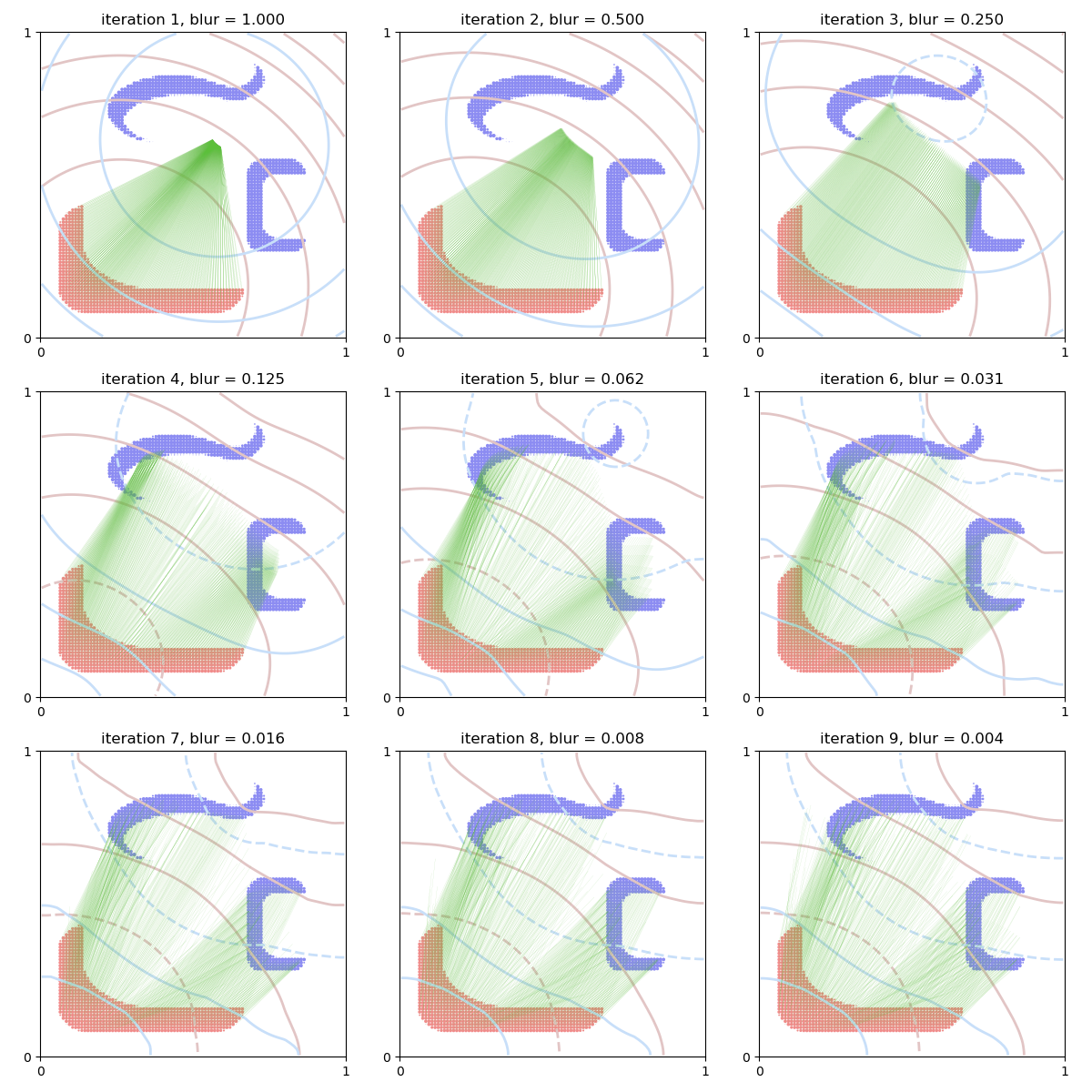
The entropic bias. In the first round of figures, we focus on the classic, biased loss

\[\text{OT}_\varepsilon(\alpha,\beta)~=~ \langle \alpha, f\rangle + \langle\beta,g\rangle,\]

where \(f\) and \(g\) are solutions of the dual problem above. Displayed in the background, the dual potentials

\[f ~=~ \partial_{\alpha} \text{OT}_\varepsilon(\alpha,\beta) \qquad\text{and}\qquad g ~=~ \partial_{\beta} \text{OT}_\varepsilon(\alpha,\beta)\]

evolve from simple convolutions of the form \(\text{C}\star\alpha\), \(\text{C}\star\beta\) (when \(\varepsilon\) is large) to genuine Kantorovitch potentials (when \(\varepsilon\) tends to zero).

Unfortunately though, as was first illustrated in (Chui and Rangarajan, 2000), the \(\text{OT}_\varepsilon\) loss suffers from an entropic bias: its Lagrangian gradient \(-\tfrac{1}{\alpha_i}\partial_{x_i} \text{OT}(\alpha,\beta)\) (i.e. its gradient for the Wasserstein metric) points towards the inside of the target measure \(\beta\), as points get attracted to the Fréchet mean of their \(\varepsilon\)-targets specified by the fuzzy transport plan \(\pi\).

display_scaling(scaling=0.5, Nits=9, debias=False)

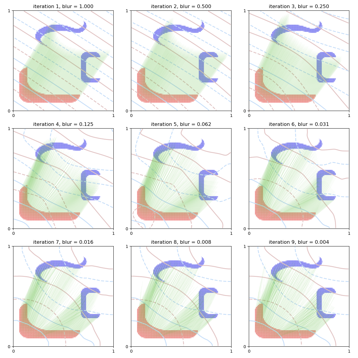
Unbiased Sinkhorn divergences. To alleviate this mode collapse phenomenon, an idea that recently emerged in the Machine Learning community is to use the unbiased Sinkhorn loss (Ramdas et al., 2015):

\[\text{S}_\varepsilon(\alpha,\beta)~=~ \text{OT}_\varepsilon(\alpha,\beta) - \tfrac{1}{2}\text{OT}_\varepsilon(\alpha,\alpha) - \tfrac{1}{2}\text{OT}_\varepsilon(\beta,\beta),\]

which interpolates between a Wasserstein distance (when \(\varepsilon \rightarrow 0\)) and a kernel norm (when \(\varepsilon \rightarrow +\infty\)). In (Feydy et al., 2018), this formula was shown to define a positive, definite, convex loss function that metrizes the convergence in law. Crucially, as detailed in (Feydy and Trouvé, 2018), it can also be written as

\[\text{S}_\varepsilon(\alpha,\beta)~=~ \langle ~\alpha~, ~\underbrace{b^{\beta\rightarrow\alpha} - a^{\alpha\leftrightarrow\alpha}}_F~\rangle + \langle ~\beta~, ~\underbrace{a^{\alpha\rightarrow\beta} - b^{\beta\leftrightarrow\beta}}_G~\rangle\]

where \((f,g) = (b^{\beta\rightarrow\alpha},a^{\alpha\rightarrow\beta})\) is a solution of \(\text{OT}_\varepsilon(\alpha,\beta)\) and \(a^{\alpha\leftrightarrow\alpha}\), \(b^{\beta\leftrightarrow\beta}\) are the unique solutions of \(\text{OT}_\varepsilon(\alpha,\alpha)\) and \(\text{OT}_\varepsilon(\beta,\beta)\) on the diagonal of the space of potential pairs.

As evidenced by the figures below, the unbiased dual potentials

\[F ~=~ \partial_{\alpha} \text{S}_\varepsilon(\alpha,\beta) \qquad\text{and}\qquad G ~=~ \partial_{\beta} \text{S}_\varepsilon(\alpha,\beta)\]

interpolate between simple linear forms (when \(\varepsilon\) is large) and genuine Kantorovitch potentials (when \(\varepsilon\) tends to zero).

A generalized Brenier map. Instead of suffering from shrinking artifacts, the Lagrangian gradient of the Sinkhorn divergence interpolates between an optimal translation and an optimal transport plan. Understood as a smooth generalization of the Brenier mapping, the displacement field

\[v(x_i) ~=~ -\tfrac{1}{\alpha_i}\partial_{x_i} \text{S}(\alpha,\beta) ~=~ -\nabla F(x_i)\]

can thus be used as a blurred transport map that registers measures up to a detail scale specified through the blur parameter.

# sphinx_gallery_thumbnail_number = 2
display_scaling(scaling=0.5, Nits=9)

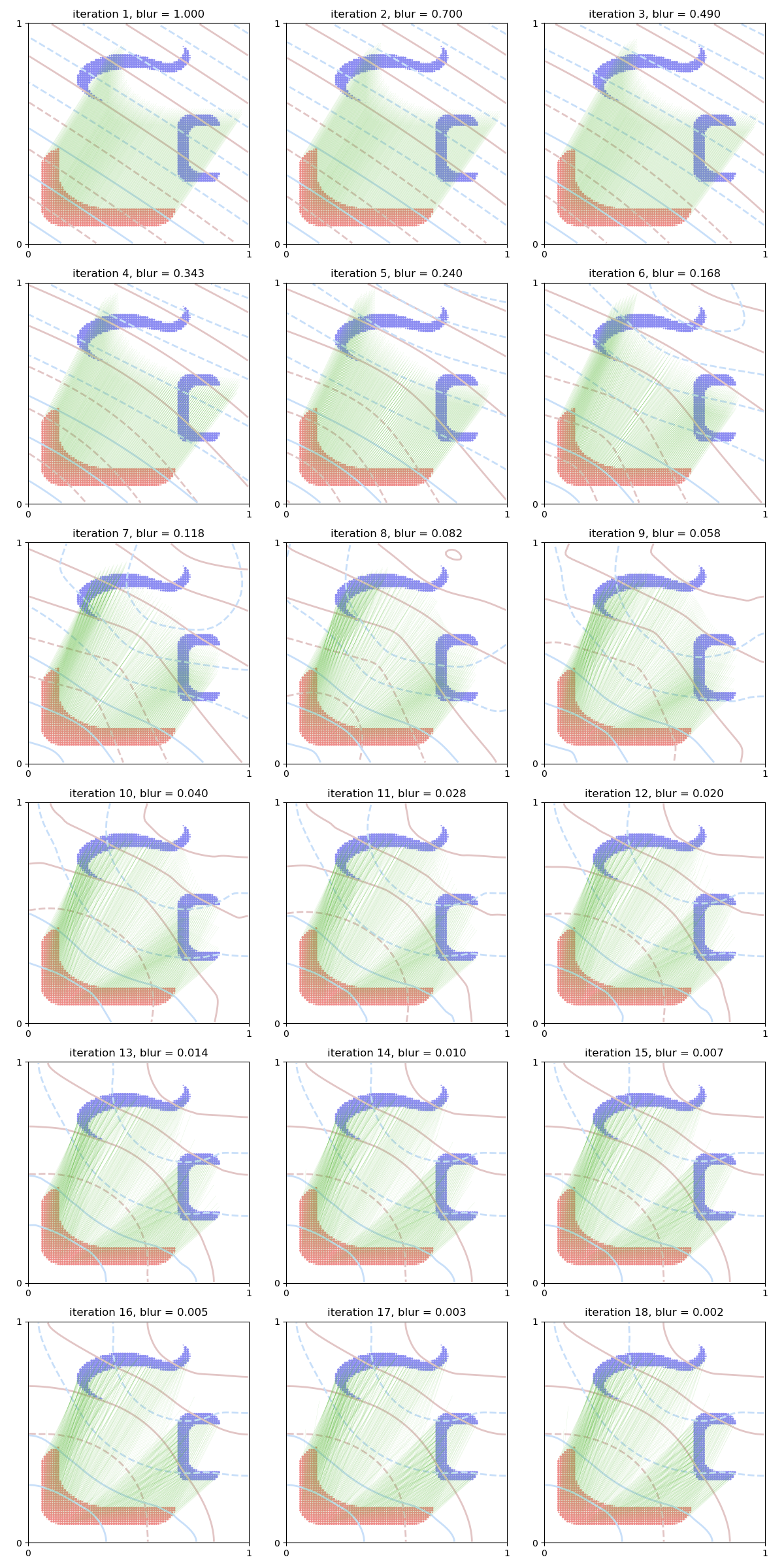
As a final note: please remember that the trade-off between speed and accuracy can be simply set by changing the value of the scaling parameter. By choosing a decay of \(.7 \simeq \sqrt{.5}\) between successive values of the blurring radius \(\sigma = \sqrt{\varepsilon}\), we effectively double the number of iterations spent to solve our dual optimization problem and thus improve the quality of our matching:

display_scaling(scaling=0.7, Nits=18)
plt.show()