2) Kernel truncation, log-linear runtimes

In the previous notebook, we’ve seen that simulated annealing could be used to define efficient coarse-to-fine solvers of the entropic \(\text{OT}_\varepsilon\) problem. Adapting ideas from (Schmitzer, 2016), we now explain how the SamplesLoss("sinkhorn", backend="multiscale") layer combines this strategy with a multiscale encoding of the input measures to compute Sinkhorn divergences in \(O(n \log(n))\) times, on the GPU.

Warning

The recent line of Stats-ML papers on entropic OT started by (Cuturi, 2013) has prioritized the theoretical study of statistical properties over computational efficiency. Consequently, in spite of their impact on fluid mechanics, computer graphics and all fields where a manifold assumption may be done on the input measures, multiscale methods have been mostly ignored by authors in the Machine Learning community.

By providing a fast discrete OT solver that relies on key ideas from both worlds, GeomLoss aims at bridging the gap between these two bodies of work. As researchers become aware of both geometric and statistical points of view on discrete OT, we will hopefully converge towards robust, efficient and well-understood generalizations of the Wasserstein distance.

Multiscale Optimal Transport

In the general case, Optimal Transport problems are linear programs that cannot be solved with less than \(O(n^2)\) operations: at the very least, the cost function \(\text{C}\) should be evaluated on all pairs of points! But fortunately, when the data is intrinsically low-dimensional, efficient algorithms allow us to leverage the structure of the cost matrix \((\text{C}(x_i,y_j))_{i,j}\) to prune out useless computations and reach the optimal \(O(n \log(n))\) complexity that is commonly found in physics and computer graphics.

As far as I can tell, the first multiscale OT solver was presented in a seminal paper of Quentin Mérigot, (Mérigot, 2011). In the simple case of entropic OT, which was best studied in (Schmitzer, 2016), multiscale schemes rely on two key observations made on the \(\varepsilon\)-scaling descent:

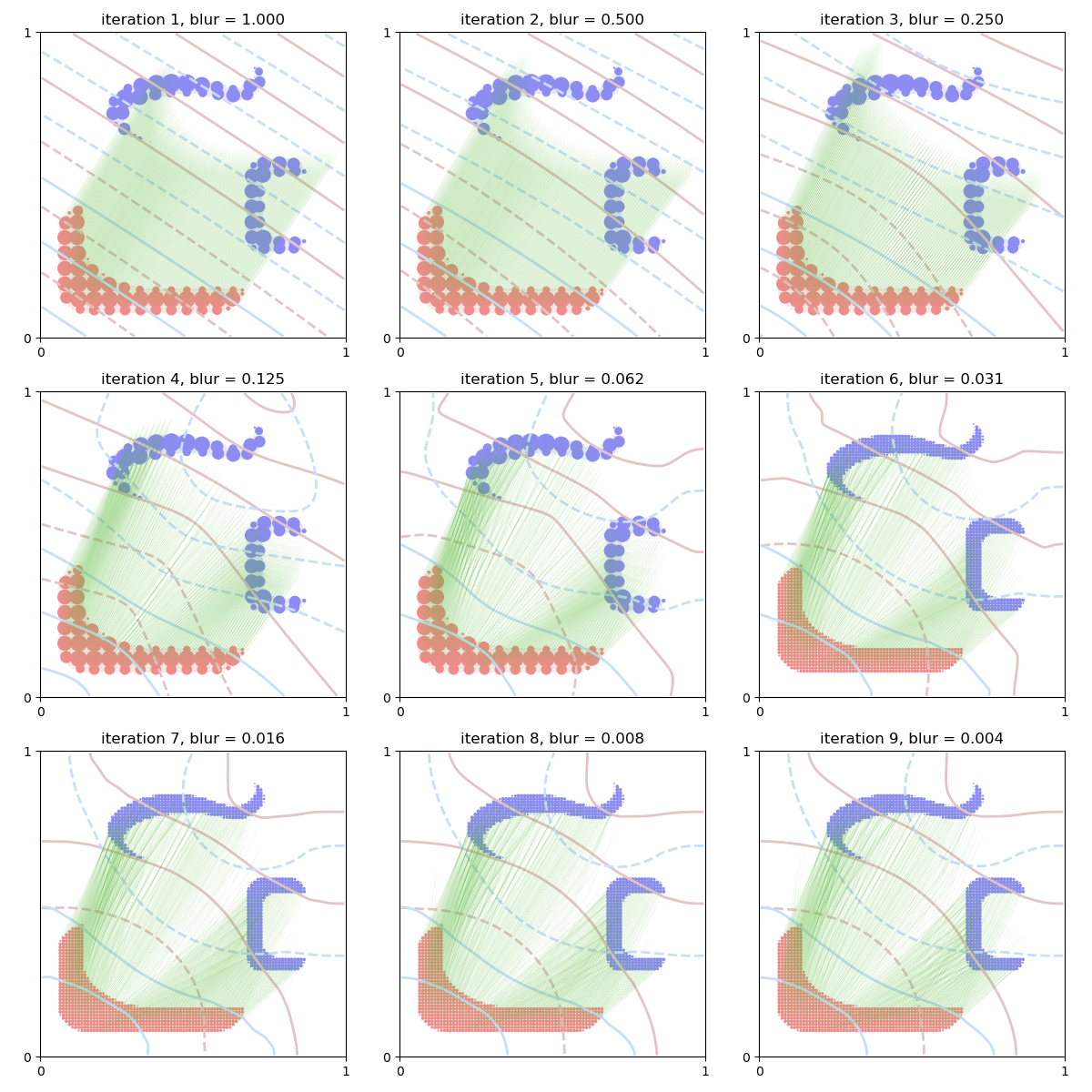
1. When the blurring radius \(\sigma = \varepsilon^{1/p}\) is large, the dual potentials \(f\) and \(g\) define smooth functions on the ambient space, that can be described accurately with coarse samples at scale \(\sigma\). The first few iterations of the Sinkhorn loop could thus be performed quickly, on sub-sampled point clouds \(\tilde{x}_i\) and \(\tilde{y}_j\) computed with an appropriate clustering method.

2. The fuzzy transport plans \(\pi_\varepsilon\), solutions of the primal problem \(\text{OT}_\varepsilon(\alpha,\beta)\) for decreasing values of \(\varepsilon\) typically define a nested sequence of measures on the product space \(\alpha\otimes \beta\). Informally, we may assume that

   \[\varepsilon ~<~\varepsilon' ~\Longrightarrow~ \text{Supp}(\pi_\varepsilon) ~\subset~ \text{Supp}(\pi_{\varepsilon'}).\]

   If \((f_\varepsilon,g_\varepsilon)\) denotes an optimal dual pair for the coarse problem \(\text{OT}_\varepsilon(\tilde{\alpha},\tilde{\beta})\) at temperature \(\varepsilon\), we know that the effective support of

   \[\pi_\varepsilon ~=~ \exp \tfrac{1}{\varepsilon}[ f_\varepsilon \oplus g_\varepsilon - \text{C}] \,\cdot\, \tilde{\alpha}\otimes\tilde{\beta}\]

   is typically restricted to pairs of coarse points \((\tilde{x}_i,\tilde{y}_j)\), i.e. pairs of clusters, such that

   \[f_\varepsilon(\tilde{x}_i) + g_\varepsilon(\tilde{y}_j) ~\geqslant~ \text{C}(\tilde{x}_i, \tilde{y}_j) \,-\,5\varepsilon.\]

   By leveraging this coarse-level information to prune out computations at a finer level (kernel truncation), we may perform a full Sinkhorn loop without ever computing point-to-point interactions that would have a negligible impact on the updates of the dual potentials.

The GeomLoss implementation

In practice, the SamplesLoss("sinkhorn", backend="multiscale") layer relies on a single loop that differs significantly from Bernhard Schmitzer’s reference CPU implementation. Some modifications were motivated by mathematical insights, and may be relevant for all entropic OT solvers:

• As discussed in the previous notebook, if the optional argument debias is set to True (the default behavior), we compute the unbiased dual potentials \(F\) and \(G\) which correspond to the positive and definite Sinkhorn divergence \(\text{S}_\varepsilon\).

• For the sake of numerical stability, all computations are performed in the log-domain. We rely on efficient, online Log-Sum-Exp routines provided by the KeOps library.

• For the sake of symmetry, we use averaged updates on the dual potentials \(f\) and \(g\) instead of the standard alternate iterations of the Sinkhorn algorithm. This allows us to converge (much) faster when the two input measures are close to each other, and we also make sure that:

  \[\text{S}_\varepsilon(\alpha,\beta)=\text{S}_\varepsilon(\beta,\alpha), ~~\text{S}_\varepsilon(\alpha,\alpha) = 0 ~~\text{and}~~ \partial_{\alpha} \text{S}_\varepsilon(\alpha,\beta=\alpha) = 0,\]

  even after a finite number of iterations.

• When jumping from coarse to fine scales, we use the “true”, closed-form expression of our dual potentials instead of Bernhard’s (simplistic) piecewise-constant extrapolation rule. In practice, this simple trick allows us to be much more aggressive during the descent and only spend one iteration per value of the temperature \(\varepsilon\).

• Our gradients are computed using an explicit formula, at convergence, thus bypassing a naive backpropagation through the whole Sinkhorn loop.

Other tricks are more hardware-dependent, and result from trade-offs between computation times and memory accesses on the GPU:

• CPU implementations typically rely on lists and sparse matrices; but for the sake of performances on GPUs, we combine a sorting pass with a block-sparse truncation scheme that enforces contiguity in memory. Once again, we rely on CUDA codes that are abstracted and documented in the KeOps library.

• For the sake of simplicity, I only implemented a two-scale algorithm which performs well when working with 50,000-500,000 samples per measure. On the GPU, (semi) brute-force methods tend to have less overhead than finely crafted tree-like methods, and I found that using a single coarse scale is a good compromise for this range of problems. In the future, I may try to extend this code to let it scale on clouds with more than a million of points… but I don’t know if this would be of use to anybody!

• As discussed in the next notebook, our implementation is not limited to dimensions 2 and 3. Feel free to use this layer in conjunction with your favorite clustering scheme, e.g. a straightforward K-means in dimension 100, and expect decent speed-ups if your data is intrinsically low-dimensional.

Crucially, GeomLoss does not perform any of the sanity checks described in Bernhard’s paper (e.g. on updates of the kernel truncation mask), which allow him to guarantee the correctness of his solution to the \(\text{OT}_\varepsilon\) problem. Running these tests during the descent would induce a significant overhead, for little practical impact.

Note

As of today, the “multiscale” backend of the SamplesLoss layer should thus be understood as a pragmatic, GPU-friendly algorithm that provides quick estimates of the Wasserstein distance and gradient on large-scale problems, without guarantees. I find it good enough for most measure-fitting applications… But my personal experience is far from covering all use-cases. If you observe weird behaviors on your own range of transportation problems, please let me know!

Setup

Standard imports:

import numpy as np
import matplotlib.pyplot as plt
import time
import torch
import os
from torch.autograd import grad

use_cuda = torch.cuda.is_available()
dtype = torch.cuda.FloatTensor if use_cuda else torch.FloatTensor

Display routines:

from imageio import imread


def load_image(fname):
    img = np.mean(imread(fname), axis=2)  # Grayscale
    img = (img[::-1, :]) / 255.0
    return 1 - img


def draw_samples(fname, sampling, dtype=dtype):
    A = load_image(fname)
    A = A[::sampling, ::sampling]
    A[A <= 0] = 1e-8

    a_i = A.ravel() / A.sum()

    x, y = np.meshgrid(
        np.linspace(0, 1, A.shape[0]),
        np.linspace(0, 1, A.shape[1]),
        indexing="xy",
    )
    x += 0.5 / A.shape[0]
    y += 0.5 / A.shape[1]

    x_i = np.vstack((x.ravel(), y.ravel())).T

    return torch.from_numpy(a_i).type(dtype), torch.from_numpy(x_i).contiguous().type(
        dtype
    )


def display_potential(ax, F, color, nlines=21):
    # Assume that the image is square...
    N = int(np.sqrt(len(F)))
    F = F.view(N, N).detach().cpu().numpy()
    F = np.nan_to_num(F)

    # And display it with contour lines:
    levels = np.linspace(-1, 1, nlines)
    ax.contour(
        F,
        origin="lower",
        linewidths=2.0,
        colors=color,
        levels=levels,
        extent=[0, 1, 0, 1],
    )


def display_samples(ax, x, weights, color, v=None):
    x_ = x.detach().cpu().numpy()
    weights_ = weights.detach().cpu().numpy()

    weights_[weights_ < 1e-5] = 0
    ax.scatter(x_[:, 0], x_[:, 1], 10 * 500 * weights_, color, edgecolors="none")

    if v is not None:
        v_ = v.detach().cpu().numpy()
        ax.quiver(
            x_[:, 0],
            x_[:, 1],
            v_[:, 0],
            v_[:, 1],
            scale=1,
            scale_units="xy",
            color="#5CBF3A",
            zorder=3,
            width=2.0 / len(x_),
        )

Dataset

Our source and target samples are drawn from measures whose densities are stored in simple PNG files. They allow us to define a pair of discrete probability measures:

\[\alpha ~=~ \sum_{i=1}^N \alpha_i\,\delta_{x_i}, ~~~ \beta ~=~ \sum_{j=1}^M \beta_j\,\delta_{y_j}.\]

sampling = 10 if not use_cuda else 2

A_i, X_i = draw_samples("data/ell_a.png", sampling)
B_j, Y_j = draw_samples("data/ell_b.png", sampling)

/home/code/geomloss/geomloss/examples/sinkhorn_multiscale/plot_kernel_truncation.py:185: DeprecationWarning: Starting with ImageIO v3 the behavior of this function will switch to that of iio.v3.imread. To keep the current behavior (and make this warning disappear) use `import imageio.v2 as imageio` or call `imageio.v2.imread` directly.
  img = np.mean(imread(fname), axis=2)  # Grayscale

Scaling strategy

We now display the behavior of the Sinkhorn loss across our iterations.

from pykeops.torch.cluster import grid_cluster, cluster_ranges_centroids
from geomloss import SamplesLoss


scaling, Nits = 0.5, 9
cluster_scale = 0.1 if not use_cuda else 0.05

plt.figure(figsize=((12, ((Nits - 1) // 3 + 1) * 4)))

for i in range(Nits):
    blur = scaling ** i
    Loss = SamplesLoss(
        "sinkhorn",
        p=2,
        blur=blur,
        diameter=1.0,
        cluster_scale=cluster_scale,
        scaling=scaling,
        backend="multiscale",
    )

    # Create a copy of the data...
    a_i, x_i = A_i.clone(), X_i.clone()
    b_j, y_j = B_j.clone(), Y_j.clone()

    # And require grad:
    a_i.requires_grad = True
    x_i.requires_grad = True
    b_j.requires_grad = True

    # Compute the loss + gradients:
    Loss_xy = Loss(a_i, x_i, b_j, y_j)
    [F_i, G_j, dx_i] = grad(Loss_xy, [a_i, b_j, x_i])

    #  The generalized "Brenier map" is (minus) the gradient of the Sinkhorn loss
    # with respect to the Wasserstein metric:
    BrenierMap = -dx_i / (a_i.view(-1, 1) + 1e-7)

    # Compute the coarse measures for display ----------------------------------

    x_lab = grid_cluster(x_i, cluster_scale)
    _, x_c, a_c = cluster_ranges_centroids(x_i, x_lab, weights=a_i)

    y_lab = grid_cluster(y_j, cluster_scale)
    _, y_c, b_c = cluster_ranges_centroids(y_j, y_lab, weights=b_j)

    # Fancy display: -----------------------------------------------------------

    ax = plt.subplot(((Nits - 1) // 3 + 1), 3, i + 1)
    ax.scatter([10], [10])  # shameless hack to prevent a slight change of axis...

    display_potential(ax, G_j, "#E2C5C5")
    display_potential(ax, F_i, "#C8DFF9")

    if blur > cluster_scale:
        display_samples(ax, y_j, b_j, [(0.55, 0.55, 0.95, 0.2)])
        display_samples(ax, x_i, a_i, [(0.95, 0.55, 0.55, 0.2)], v=BrenierMap)
        display_samples(ax, y_c, b_c, [(0.55, 0.55, 0.95)])
        display_samples(ax, x_c, a_c, [(0.95, 0.55, 0.55)])

    else:
        display_samples(ax, y_j, b_j, [(0.55, 0.55, 0.95)])
        display_samples(ax, x_i, a_i, [(0.95, 0.55, 0.55)], v=BrenierMap)

    ax.set_title("iteration {}, blur = {:.3f}".format(i + 1, blur))

    ax.set_xticks([0, 1])
    ax.set_yticks([0, 1])
    ax.axis([0, 1, 0, 1])
    ax.set_aspect("equal", adjustable="box")

plt.tight_layout()
plt.show()

/opt/conda/lib/python3.10/site-packages/torch/functional.py:504: UserWarning: torch.meshgrid: in an upcoming release, it will be required to pass the indexing argument. (Triggered internally at /opt/conda/conda-bld/pytorch_1678402411778/work/aten/src/ATen/native/TensorShape.cpp:3483.)
  return _VF.meshgrid(tensors, **kwargs)  # type: ignore[attr-defined]

Analogy with a Quicksort algorithm

In some sense, Optimal Transport can be understood as a generalization of sorting problems as we “index” a weighted point cloud with another one. But how far can we go with this analogy?

In dimension 1, when \(p \geqslant 1\), the optimal Monge map can be computed through a simple sorting pass on the data with \(O(n \log(n))\) complexity. At the other end of the spectrum, generic OT problems on high-dimensional, scattered point clouds have little to no structure and cannot be solved with less than \(O(n^2)\) or \(O(n^3)\) operations.

From this perspective, multiscale OT solvers should thus be understood as multi-dimensional Quicksort algorithms, with coarse cluster centroids and their targets playing the part of median pivots. With its pragmatic GPU implementation, GeomLoss has simply delivered on the promise made by a long line of research papers: when your data is intrinsically low-dimensional, the runtime needed to compute a Wasserstein distance should be closer to a \(O(n \log(n))\) than to a \(O(n^2)\).