3) Optimal Transport in high dimension

Let’s use a custom clustering scheme to generalize the multiscale Sinkhorn algorithm to high-dimensional settings.

Setup

Standard imports:

import numpy as np
import matplotlib.pyplot as plt
import time

import torch
from geomloss import SamplesLoss

use_cuda = torch.cuda.is_available()
dtype = torch.cuda.FloatTensor if use_cuda else torch.FloatTensor


def display_4d_samples(ax1, ax2, x, color):
    x_ = x.detach().cpu().numpy()
    if not type(color) in [str, list]:
        color = color.detach().cpu().numpy()
    ax1.scatter(
        x_[:, 0], x_[:, 1], 25 * 500 / len(x_), color, edgecolors="none", cmap="tab10"
    )
    ax2.scatter(
        x_[:, 2], x_[:, 3], 25 * 500 / len(x_), color, edgecolors="none", cmap="tab10"
    )

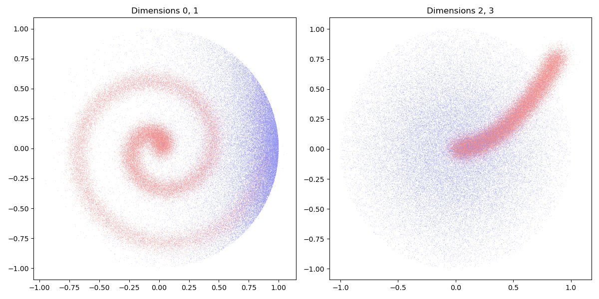
Dataset. Our source and target samples are drawn from (noisy) discrete sub-manifolds in ${\mathbb{R}}^4$. They allow us to define a pair of discrete probability measures:

$$\alpha =\frac{1}{N}\sum _{i=1}^N{\delta }_{x_i},\beta =\frac{1}{M}\sum _{j=1}^M{\delta }_{y_j}.$$

N, M = (100, 100) if not use_cuda else (50000, 50000)

# Generate some kind of 4d-helix:
t = torch.linspace(0, 2 * np.pi, N).type(dtype)
X_i = (
    torch.stack((t * (2 * t).cos() / 7, t * (2 * t).sin() / 7, t / 7, t**2 / 50))
    .t()
    .contiguous()
)
X_i = X_i + 0.05 * torch.randn(N, 4).type(dtype)  # + some noise

# The y_j's are sampled non-uniformly on the unit sphere of R^4:
Y_j = torch.randn(M, 4).type(dtype)
Y_j[:, 0] += 2
Y_j = Y_j / (1e-4 + Y_j.norm(dim=1, keepdim=True))

We display our 4d-samples using two 2d-views:

plt.figure(figsize=(12, 6))

ax1 = plt.subplot(1, 2, 1)
plt.title("Dimensions 0, 1")
ax2 = plt.subplot(1, 2, 2)
plt.title("Dimensions 2, 3")

display_4d_samples(ax1, ax2, X_i, [(0.95, 0.55, 0.55)])
display_4d_samples(ax1, ax2, Y_j, [(0.55, 0.55, 0.95)])

plt.tight_layout()

/home/code/geomloss/geomloss/examples/sinkhorn_multiscale/plot_optimal_transport_cluster.py:31: UserWarning: No data for colormapping provided via 'c'. Parameters 'cmap' will be ignored
  ax1.scatter(
/home/code/geomloss/geomloss/examples/sinkhorn_multiscale/plot_optimal_transport_cluster.py:34: UserWarning: No data for colormapping provided via 'c'. Parameters 'cmap' will be ignored
  ax2.scatter(

Online Sinkhorn algorithm

When working with large point clouds in dimension > 3, the SamplesLoss("sinkhorn") layer relies on an online implementation of the Sinkhorn algorithm (in the log-domain, with $\epsilon$-scaling) which computes softmin reductions on-the-fly, with a linear memory footprint:

from geomloss import SamplesLoss

# Compute the Wasserstein-2 distance between our samples,
# with a small blur radius and a conservative value of the
# scaling "decay" coefficient (.8 is pretty close to 1):
Loss = SamplesLoss("sinkhorn", p=2, blur=0.05, scaling=0.8)

start = time.time()
Wass_xy = Loss(X_i, Y_j)
if use_cuda:
    torch.cuda.synchronize()
end = time.time()

print(
    "Wasserstein distance: {:.3f}, computed in {:.3f}s.".format(
        Wass_xy.item(), end - start
    )
)

Wasserstein distance: 0.510, computed in 0.517s.

Multiscale Sinkhorn algorithm

Thanks to the $\epsilon$-scaling heuristic, this online backend already outperforms a naive implementation of the Sinkhorn/Auction algorithm by a factor ~10, for comparable values of the blur parameter. But we can go further.

A key insight from recent works on computational Optimal Transport is that the dual optimization problem on the potentials (or prices) $f$ and $g$ can often be solved efficiently in a coarse-to-fine fashion, using a clever subsampling of the input measures in the first iterations of the $\epsilon$-scaling descent.

For regularized Optimal Transport, the main reference on the subject is (Schmitzer, 2016) which combines an octree-like encoding with a kernel truncation (pruning) scheme to achieve log-linear complexity. Going further, (Gerber and Maggioni, 2017) generalize these ideas to high-dimensional scenarios, using a clever multiscale decomposition that relies on the manifold-like structure of the data - if any.

Leveraging the block-sparse routines of the KeOps library, the multiscale backend of the SamplesLoss("sinkhorn") layer provides the first GPU implementation of these strategies. In dimensions 1, 2 and 3, clustering is automatically performed using a straightforward cubic grid. But in the general case, clustering information can simply be provided through a vector of labels, alongside the weights and samples’ locations.

Clustering in high-dimension. In this tutorial, we rely on an off-the-shelf K-means clustering, copy-pasted from the examples gallery of the KeOps library: feel free to replace it with a more clever scheme if needed!

from pykeops.torch import generic_argmin


def KMeans(x, K=10, Niter=10, verbose=True):
    N, D = x.shape  # Number of samples, dimension of the ambient space

    # Define our KeOps CUDA kernel:
    nn_search = generic_argmin(  # Argmin reduction for generic formulas:
        "SqDist(x,y)",  # A simple squared L2 distance
        "ind = Vi(1)",  # Output one index per "line" (reduction over "j")
        "x = Vi({})".format(D),  # 1st arg: one point per "line"
        "y = Vj({})".format(D),
    )  # 2nd arg: one point per "column"

    # K-means loop:
    # - x  is the point cloud,
    # - cl is the vector of class labels
    # - c  is the cloud of cluster centroids
    start = time.time()

    # Simplistic random initialization for the cluster centroids:
    perm = torch.randperm(N)
    idx = perm[:K]
    c = x[idx, :].clone()

    for i in range(Niter):
        cl = nn_search(x, c).view(-1)  # Points -> Nearest cluster
        Ncl = torch.bincount(cl).type(dtype)  # Class weights
        for d in range(D):  # Compute the cluster centroids with torch.bincount:
            c[:, d] = torch.bincount(cl, weights=x[:, d]) / Ncl
    if use_cuda:
        torch.cuda.synchronize()
    end = time.time()
    if verbose:
        print("KMeans performed in {:.3f}s.".format(end - start))

    return cl, c


lab_i, c_i = KMeans(X_i, K=100 if use_cuda else 10)
lab_j, c_j = KMeans(Y_j, K=400 if use_cuda else 10)

KMeans performed in 0.008s.
KMeans performed in 0.008s.

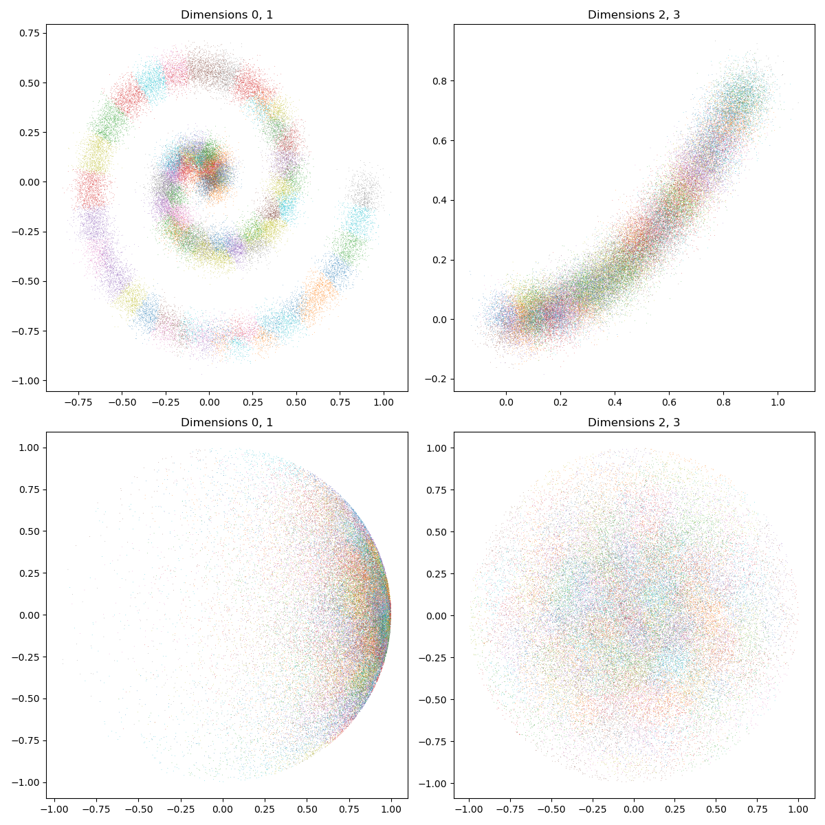
The average cluster size can be computed with one line of code:

std_i = ((X_i - c_i[lab_i, :]) ** 2).sum(1).mean().sqrt()
std_j = ((Y_j - c_j[lab_j, :]) ** 2).sum(1).mean().sqrt()

print(
    "Our clusters have standard deviations of {:.3f} and {:.3f}.".format(std_i, std_j)
)

Our clusters have standard deviations of 0.082 and 0.134.

As expected, our samples are now distributed in small, convex clusters that partition the input data:

# sphinx_gallery_thumbnail_number = 2
plt.figure(figsize=(12, 12))

ax1 = plt.subplot(2, 2, 1)
plt.title("Dimensions 0, 1")
ax2 = plt.subplot(2, 2, 2)
plt.title("Dimensions 2, 3")
ax3 = plt.subplot(2, 2, 3)
plt.title("Dimensions 0, 1")
ax4 = plt.subplot(2, 2, 4)
plt.title("Dimensions 2, 3")

display_4d_samples(ax1, ax2, X_i, lab_i)
display_4d_samples(ax3, ax4, Y_j, lab_j)

plt.tight_layout()

To use this information in the multiscale Sinkhorn algorithm, we should simply provide:

• explicit labels and weights for both input measures,

• a typical cluster_scale which specifies the iteration at which the Sinkhorn loop jumps from a coarse to a fine representation of the data.

Loss = SamplesLoss(
    "sinkhorn",
    p=2,
    blur=0.05,
    scaling=0.8,
    cluster_scale=max(std_i, std_j),
    verbose=True,
)

# To specify explicit cluster labels, SamplesLoss also requires
# explicit weights. Let's go with the default option - a uniform distribution:
a_i = torch.ones(N).type(dtype) / N
b_j = torch.ones(M).type(dtype) / M

start = time.time()
# 6 args -> labels_i, weights_i, locations_i, labels_j, weights_j, locations_j
Wass_xy = Loss(lab_i, a_i, X_i, lab_j, b_j, Y_j)
if use_cuda:
    torch.cuda.synchronize()
end = time.time()

100x400 clusters, computed at scale = 0.134
Successive scales :  4.022, 4.022, 3.217, 2.574, 2.059, 1.647, 1.318, 1.054, 0.843, 0.675, 0.540, 0.432, 0.345, 0.276, 0.221, 0.177, 0.142, 0.113, 0.091, 0.072, 0.058, 0.050
Jump from coarse to fine between indices 16 (σ=0.142) and 17 (σ=0.113).
Keep 13469/40000 = 33.7% of the coarse cost matrix.
Keep 2772/10000 = 27.7% of the coarse cost matrix.
Keep 28490/160000 = 17.8% of the coarse cost matrix.

That’s it! As expected, leveraging the structure of the data has allowed us to gain another ~10 speedup on large-scale transportation problems:

print(
    "Wasserstein distance: {:.3f}, computed in {:.3f}s.".format(
        Wass_xy.item(), end - start
    )
)


plt.show()

Wasserstein distance: 0.510, computed in 0.090s.