Block-sparse reductions

This script showcases the use of the optional ranges argument to compute block-sparse reductions with sub-quadratic time complexity.

Setup

Standard imports:

import time

import numpy as np
import torch
from matplotlib import pyplot as plt

from pykeops.torch import LazyTensor

nump = lambda t: t.cpu().numpy()
use_cuda = torch.cuda.is_available()
dtype = torch.cuda.FloatTensor if use_cuda else torch.FloatTensor

Define our dataset: two point clouds on the unit square.

M, N = (5000, 5000) if use_cuda else (2000, 2000)

t = torch.linspace(0, 2 * np.pi, M + 1)[:-1]
x = torch.stack((0.4 + 0.4 * (t / 7) * t.cos(), 0.5 + 0.3 * t.sin()), 1)
x = x + 0.01 * torch.randn(x.shape)
x = x.type(dtype)

y = torch.randn(N, 2).type(dtype)
y = y / 10 + dtype([0.6, 0.6])

Computing a block-sparse reduction

On the GPU, contiguous memory accesses are key to high performances. To enable the implementation of algorithms with sub-quadratic time complexity under this constraint, KeOps provides access to block-sparse reduction routines through the optional ranges argument, which is supported by torch.Genred and all its children.

Pre-processing

To leverage this feature through the pykeops.torch API, the first step is to clusterize your data into groups which should neither be too small (performances on clusters with less than ~200 points each are suboptimal) nor too many (the from_matrix() pre-processor can become a bottleneck when working with >2,000 clusters per point cloud).

In this tutorial, we use the grid_cluster() routine which simply groups points into cubic bins of arbitrary size:

from pykeops.torch.cluster import grid_cluster

eps = 0.05  # Size of our square bins

if use_cuda:
    torch.cuda.synchronize()
Start = time.time()
start = time.time()
x_labels = grid_cluster(x, eps)  # class labels
y_labels = grid_cluster(y, eps)  # class labels
if use_cuda:
    torch.cuda.synchronize()
end = time.time()
print("Perform clustering       : {:.4f}s".format(end - start))

Perform clustering       : 0.0241s

Once (integer) cluster labels have been computed, we can compute the centroids and memory footprint of each class:

from pykeops.torch.cluster import cluster_ranges_centroids

# Compute one range and centroid per class:
start = time.time()
x_ranges, x_centroids, _ = cluster_ranges_centroids(x, x_labels)
y_ranges, y_centroids, _ = cluster_ranges_centroids(y, y_labels)
if use_cuda:
    torch.cuda.synchronize()
end = time.time()
print("Compute ranges+centroids : {:.4f}s".format(end - start))

Compute ranges+centroids : 0.0040s

Finally, we can sort our points according to their labels, making sure that all clusters are stored contiguously in memory:

from pykeops.torch.cluster import sort_clusters

start = time.time()
x, x_labels = sort_clusters(x, x_labels)
y, y_labels = sort_clusters(y, y_labels)
if use_cuda:
    torch.cuda.synchronize()
end = time.time()
print("Sort the points          : {:.4f}s".format(end - start))

Sort the points          : 0.0137s

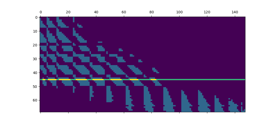
Cluster-Cluster binary mask

The key idea behind KeOps’s block-sparsity mode is that as soon as data points are sorted, we can manage the reduction scheme through a small, coarse boolean mask whose values encode whether or not we should perform computations at a finer scale.

In this example, we compute a simple Gaussian convolution of radius \(\sigma\) and decide to skip points-to-points interactions between blocks whose centroids are further apart than \(4\sigma\), as \(\exp(- (4\sigma)^2 / 2\sigma^2 ) = e^{-8} \ll 1\), with 99% of the mass of a Gaussian kernel located in the \(3\sigma\) range.

sigma = 0.05  # Characteristic length of interaction
start = time.time()

# Compute a coarse Boolean mask:
D = ((x_centroids[:, None, :] - y_centroids[None, :, :]) ** 2).sum(2)
keep = D < (4 * sigma) ** 2

To turn this mask into a set of integer Tensors which is more palatable to KeOps’s low-level CUDA API, we then use the from_matrix routine…

from pykeops.torch.cluster import from_matrix

ranges_ij = from_matrix(x_ranges, y_ranges, keep)

if use_cuda:
    torch.cuda.synchronize()
end = time.time()
print("Process the ranges       : {:.4f}s".format(end - start))

if use_cuda:
    torch.cuda.synchronize()
End = time.time()
t_cluster = End - Start
print("Total time (synchronized): {:.4f}s".format(End - Start))
print("")

Process the ranges       : 0.0024s
Total time (synchronized): 0.0460s

And we’re done: here is the ranges argument that can be fed to the KeOps reduction routines! For large point clouds, we can expect a speed-up that is directly proportional to the ratio of mass between our fine binary mask (encoded in ranges_ij) and the full, N-by-M kernel matrix:

areas = (x_ranges[:, 1] - x_ranges[:, 0])[:, None] * (y_ranges[:, 1] - y_ranges[:, 0])[
    None, :
]
total_area = areas.sum().item()  # should be equal to N*M
sparse_area = areas[keep].sum().item()
print(
    "We keep {:.2e}/{:.2e} = {:2d}% of the original kernel matrix.".format(
        sparse_area, total_area, int(100 * sparse_area / total_area)
    )
)
print("")

We keep 3.52e+06/2.50e+07 = 14% of the original kernel matrix.

Benchmark a block-sparse Gaussian convolution

Define a Gaussian kernel matrix from 2d point clouds:

x_, y_ = x / sigma, y / sigma
x_i, y_j = LazyTensor(x_[:, None, :]), LazyTensor(y_[None, :, :])
D_ij = ((x_i - y_j) ** 2).sum(dim=2)  # Symbolic (M,N,1) matrix of squared distances
K = (-D_ij / 2).exp()  # Symbolic (M,N,1) Gaussian kernel matrix

And create a random signal supported by the points \(y_j\):

b = torch.randn(N, 1).type(dtype)

Compare the performances of our block-sparse code with those of a dense implementation, on both CPU and GPU backends:

Note

The standard KeOps routine are already very efficient: on the GPU, speed-ups with multiscale, block-sparse schemes only start to kick on around the “20,000 points” mark as the skipped computations make up for the clustering and branching overheads.

backend = "GPU" if use_cuda else "CPU"

# GPU warm-up:
a = K @ b

start = time.time()
a_full = K @ b
end = time.time()
t_full = end - start
print(" Full  convolution, {} backend: {:2.4f}s".format(backend, end - start))

start = time.time()
K.ranges = ranges_ij
a_sparse = K @ b
end = time.time()
t_sparse = end - start
print("Sparse convolution, {} backend: {:2.4f}s".format(backend, end - start))
print(
    "Relative time : {:3d}% ({:3d}% including clustering), ".format(
        int(100 * t_sparse / t_full), int(100 * (t_sparse + t_cluster) / t_full)
    )
)
print(
    "Relative error:   {:3.4f}%".format(
        100 * (a_sparse - a_full).abs().sum() / a_full.abs().sum()
    )
)
print("")

 Full  convolution, GPU backend: 0.0005s
Sparse convolution, GPU backend: 0.0009s
Relative time : 179% (9269% including clustering),
Relative error:   0.2807%

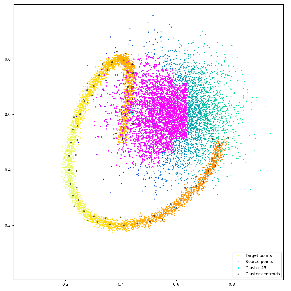
Fancy visualization: we display our coarse binary mask and highlight one of its lines, that corresponds to the cyan cluster and its magenta neighbors:

# Find the cluster centroid which is closest to the (.43,.6) point:
dist_target = ((x_centroids - torch.Tensor([0.43, 0.6]).type_as(x_centroids)) ** 2).sum(
    1
)
clust_i = torch.argmin(dist_target)

if M + N <= 500000:
    ranges_i, slices_j, redranges_j = ranges_ij[0:3]
    start_i, end_i = ranges_i[clust_i]  # Indices of the points that make up our cluster
    start, end = (
        slices_j[clust_i - 1],
        slices_j[clust_i],
    )  # Ranges of the cluster's neighbors

    keep = nump(keep.float())
    keep[clust_i] += 2

    plt.ion()
    plt.matshow(keep)

    plt.figure(figsize=(10, 10))

    x, x_labels, x_centroids = nump(x), nump(x_labels), nump(x_centroids)
    y, y_labels, y_centroids = nump(y), nump(y_labels), nump(y_centroids)

    plt.scatter(
        x[:, 0],
        x[:, 1],
        c=x_labels,
        cmap=plt.cm.Wistia,
        s=25 * 500 / len(x),
        label="Target points",
    )
    plt.scatter(
        y[:, 0],
        y[:, 1],
        c=y_labels,
        cmap=plt.cm.winter,
        s=25 * 500 / len(y),
        label="Source points",
    )

    # Target clusters:
    for start_j, end_j in redranges_j[start:end]:
        plt.scatter(
            y[start_j:end_j, 0], y[start_j:end_j, 1], c="magenta", s=50 * 500 / len(y)
        )

    # Source cluster:
    plt.scatter(
        x[start_i:end_i, 0],
        x[start_i:end_i, 1],
        c="cyan",
        s=10,
        label="Cluster {}".format(clust_i),
    )

    plt.scatter(
        x_centroids[:, 0],
        x_centroids[:, 1],
        c="black",
        s=10,
        alpha=0.5,
        label="Cluster centroids",
    )

    plt.legend(loc="lower right")

    # sphinx_gallery_thumbnail_number = 2
    plt.axis("equal")
    plt.axis([0, 1, 0, 1])
    plt.tight_layout()
    plt.show(block=True)

• 
•