Kernel Interpolation with RKeOps • rkeops

Setup

library(ggplot2) # graph generation
library(dplyr)   # data.frame manipulation
library(pracma)  # to create the meshgrid
library(plotly)  # reactive graph generation
library(reshape) # matrix to data.frame reformatting

# load rkeops
library(rkeops)
# create a dedicated Python environment with reticulate (to be done only once)
reticulate::virtualenv_create("rkeops")
# activate the dedicated Python environment
reticulate::use_virtualenv(virtualenv = "rkeops", required = TRUE)
# install rkeops requirements (to be done only once)
install_rkeops()
# use 64bit floating operation precision
rkeops_use_float64()

# check rkeops install
check_rkeops()
## 'keopscore' is available.
## 'pykeops' is available.
## pyKeOps with numpy bindings is working!
## 'rkeops' is ready and working.
## [1] TRUE

# use 64bit floating operation precision
rkeops_use_float64()

For build on CRAN, use CPU computing with 2 cores:

rkeops_use_cpu(ncore = 2)

Note: you can run rkeops_use_cpu() to use all available CPU cores or rkeops_use_gpu() to enable GPU computing.

Introduction

This tutorial is highly inspired by the PyKeOps tutorial on kernel interpolation.

The goal here is to solve a linear system of the form,

\[ \begin{aligned} &a^{*} = \underset{a}{\textrm{argmin}} \frac{1}{2} \langle a, (\lambda \textrm{Id} + K_{xx})a \rangle - \langle a, b \rangle \\ \text{i.e.} \quad &a^{*} = (\lambda \textrm{Id} + K_{xx})^{-1}b \end{aligned} \]

where \(K_{xx}\) is a symmetric, positive definite matrix encoded as an RKeOps LazyTensor, and \(\lambda\) is a nonnegative regularization parameter. In the following script, we use the conjugate gradient method to solve large-scale Kriging (a.k.a. Gaussian process regression or generelized spline interpolation) problems with a linear memory footprint.

Interpolation in 1D

Generate some data:

N <- 10000 # number of samples

x <- matrix(runif(N * 1), N, 1)
pert <- matrix(runif(N * 1), N, 1) # random perturbation to create b

# Some random-ish 1D signal:
b <- x + 0.5 * sin(6 * x) + 0.1 * sin(20 * x) + 0.05 * pert

Specify our regression model - a simple Gaussian variogram or kernel matrix of deviation sigma.

gaussian_kernel <- function(x, y, sigma = 0.1) {
    x_i <- Vi(x) # symbolic 'i'-indexed matrix
    y_j <- Vj(y) # symbolic 'j'-indexed matrix
    D_ij <- sum((x_i - y_j)^2) # symbolic matrix of squared distances
    res <- exp(-D_ij / (2 * sigma^2)) # symbolic Gaussian kernel matrix
    return(res)
}

Kernel Interpolation

We implement the conjugate gradient algorithm, that includes the lambda regularization parameter.

CG_solve <- function(K, b, lambda, eps = 1e-6) {
    # ----------------------------------------------------------------
    # Conjugate gradient algorithm to solve linear systems of the form
    # (K + lambda * Id) * a = b.
    #
    # K: a LazyTensor encoding a symmetric positive definite matrix
    #       (the spectrum of the matrix must not contain zero)
    # b: a vector corresponding to the second member of the equation
    # lambda: Non-negative ridge regularization parameter
    #       (lambda = 0 means no regularization)
    # eps (default=1e-6): precision parameter
    # ----------------------------------------------------------------
    delta <- length(b) * eps^2
    a <- 0
    r <- b
    nr2 <- sum(r^2) # t(r)*r (L2-norm)
    if(nr2 < delta) {
        return(0 * r)
    }
    p <- r
    k <- 0
    while (TRUE) {
      Mp <- K %*% Vj(p) + lambda * p
      alp <- nr2 / sum(p * Mp)
      a <- a + (alp * p)
      r <- r - (alp * Mp)
      nr2new <- sum(r^2)
      if (nr2new < delta) {
          break
      }
      p <- r + (nr2new / nr2) * p
      nr2 <- nr2new
      k <- k + 1
    }
    return(a) # should be such that K%*%a + lambda * Id * a = b (eps close) 
}

Perform the Kernel interpolation, without forgetting to specify the ridge regularization parameter lambda which controls the trade-off between a perfect fit (lambda = \(0\)) and a smooth interpolation (lambda = \(+\infty\)):

K_xx <- gaussian_kernel(x, x)

lambda <- 1

start <- Sys.time()
a <- CG_solve(K_xx, b, lambda = lambda)
## Loading required namespace: testthat
end <- Sys.time()

time <- round(as.numeric(end - start), 5)

print(paste("Time to perform an RBF interpolation with",
            N,"samples in 1D:", time, "s.",
            sep = " "
            )
      )
## [1] "Time to perform an RBF interpolation with 10000 samples in 1D: 21.58736 s."

Display the (fitted) model on the unit interval:

# extrapolate on a uniform sample
t <- as.matrix(seq(from = 0, to = 1, length.out = N))

K_tx <- gaussian_kernel(t, x)
mean_t <- K_tx %*% Vj(a)

D <- as.data.frame(cbind(x, b, t, mean_t))
colnames(D) <- c("x", "b", "t", "mean_t")

# 1D plot
ggplot(aes(x = x, y = b), data = D) +
  geom_point(color = '#1193a8', alpha = 0.5, size = 0.4) +
  geom_line(aes(x = t, y = mean_t), color = 'darkred') +
  annotate("text", x = .75, y = .1,
           label = paste("Number of samples: ", N,
                         sep = "")
           ) +
  theme_bw()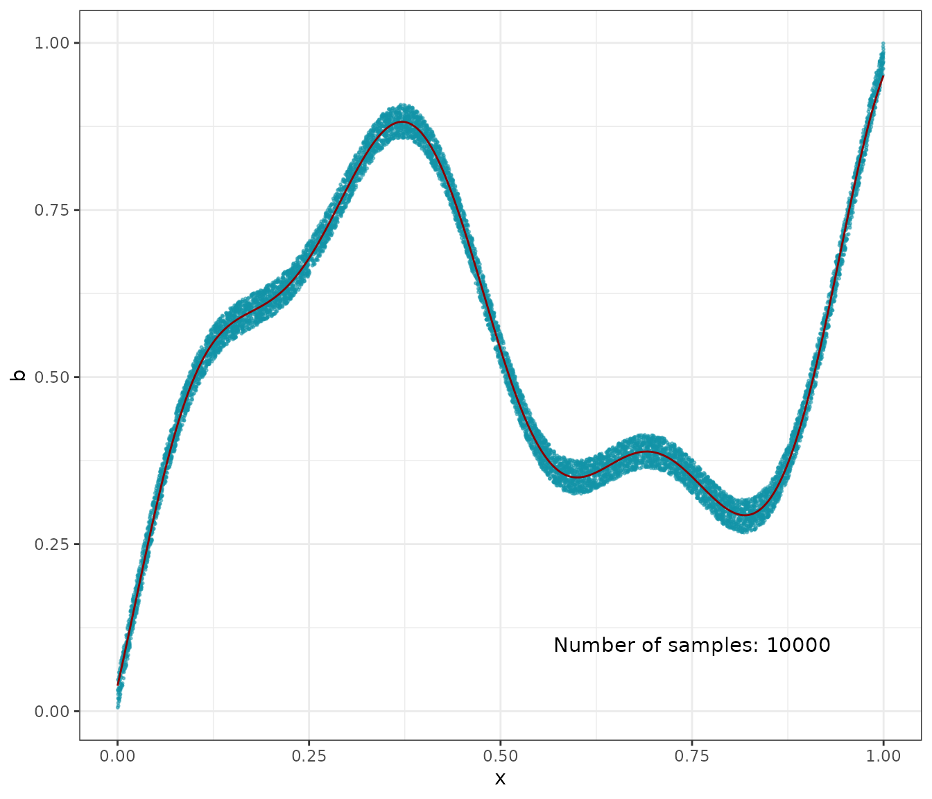

Interpolation in 2D

Generate some data:

N <- 10000
# Sampling locations:
x <- matrix(runif(N * 2), N, 2)

# Some random-ish 2D signal:
b <- as.matrix(rowSums((x - 0.5)^2))
b[b > 0.4^2] = 0
b[b < 0.3^2] = 0
b[b >= 0.3^2] = 1

pert <- matrix(runif(N * 1), N, 1) # random perturbation to create b
b <- b + 0.05 * pert

# Add 25% of outliers:
Nout <- N %/% 4
b[(length(b) - Nout + 1):length(b)] <- matrix(runif(Nout * 1), Nout, 1)

Specify our regression model - a simple Exponential variogram or Laplacian kernel matrix of deviation sigma:

laplacian_kernel <- function(x, y, sigma = 0.1) {
  x_i <- Vi(x)
  y_j <- Vj(y)
  D_ij <- sum((x_i - y_j)^2)
  res <- exp(-sqrt(D_ij) / sigma)
  return(res)
}

Perform the Kernel interpolation, without forgetting to specify the ridge regularization parameter lambda which controls the trade-off between a perfect fit (lambda = \(0\)) and a smooth interpolation (lambda = \(+\infty\)):

lambda <- 10  # Ridge regularization

start <- Sys.time()
K_xx <- laplacian_kernel(x, x)
a <- CG_solve(K_xx, b, lambda = lambda)
end <- Sys.time()

time <- round(as.numeric(end - start), 5)
print(paste("Time to perform an RBF interpolation with",
            N, "samples in 2D:", time, "s.",
            sep = " "))
## [1] "Time to perform an RBF interpolation with 10000 samples in 2D: 32.48329 s."

Interpolate and display the (fitted) model:

# Interpolate on a uniform sample:
X <- seq(from = 0, to = 1, length.out = 100)
Y <- seq(from = 0, to = 1, length.out = 100)

G <- meshgrid(X, Y)
t <- cbind(as.vector(G$X), as.vector(G$Y))

K_tx <- laplacian_kernel(t, x)
mean_t <- K_tx %*% Vj(a)

mean_t <- matrix(mean_t, 100, 100)
mean_t <- mean_t[nrow(mean_t):1, ]

# Data
data2plot_sample <- data.frame(
    X = x[,1],
    Y = x[,2],
    value = b
)

ggplot(data2plot_sample, aes(x = X, y = Y, col = value)) + 
    geom_point() +
    scale_color_gradient(low = "#C2C2C9", high = "darkred") + 
    coord_fixed() +
    theme_bw()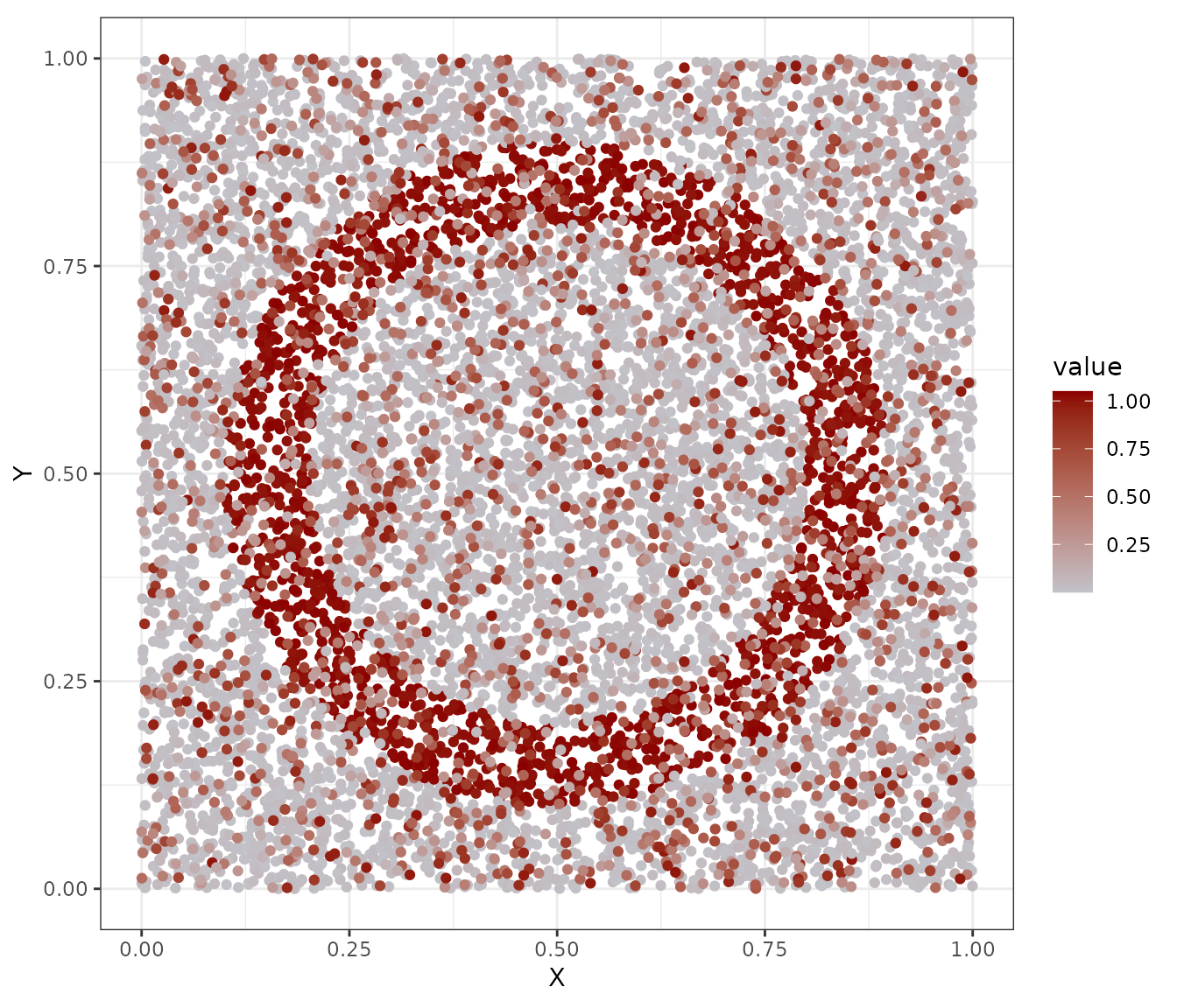

Data sample

Data sample

# Interpolation
data2plot_interpol <- reshape::melt(mean_t) %>% 
    mutate(X = X[X1], Y = Y[X2]) %>% dplyr::select(!c(X1, X2))

ggplot(data2plot_interpol, aes(x = X, y = Y, fill = value)) + 
    geom_tile() + 
    scale_fill_gradient(low = "#C2C2C9", high = "darkred") + 
    coord_fixed() +
    theme_bw()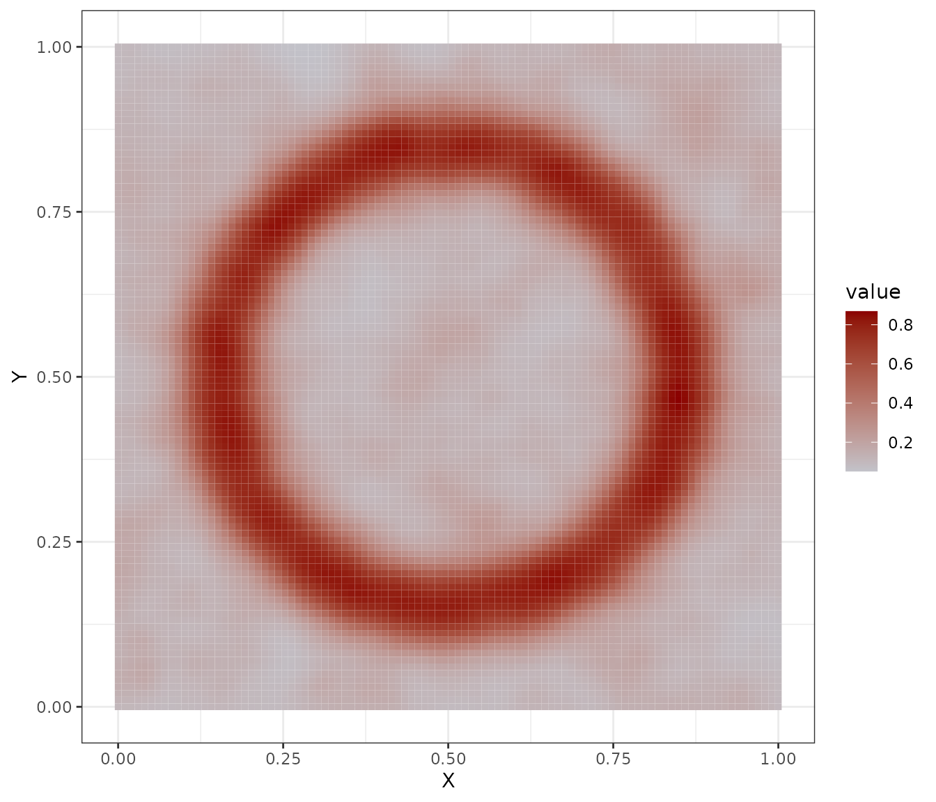

Kernel interpolation

Kernel interpolation

Plotly interactive graph:

# 2D plot: noisy samples and interpolation in the background
fig <- plot_ly(z = mean_t,
               type = "heatmap",
               colors = colorRamp(c("#C2C2C9", "darkred")),
               zsmooth ="best"
               )

fig <- fig %>% add_trace(type = "scatter",
                         x = ~(100 * x[, 1]),
                         y = ~(100 * x[, 2]),
                         mode = "markers",
                         marker = list(size = 4, color = as.vector(b))
                         )

fig <- fig %>% plotly::layout(xaxis = list(title = ""),
                      yaxis = list(title = ""))

colorbar(fig, limits = c(0, 1), x = 1, y = 0.75)