Color transfer with Optimal Transport

Let’s use the gradient of the Sinkhorn divergence to change the color palette of an image.

Setup

import numpy as np
import matplotlib.pyplot as plt
from mpl_toolkits.mplot3d import Axes3D

import time

import torch
from geomloss import SamplesLoss

use_cuda = torch.cuda.is_available()
dtype = torch.cuda.FloatTensor if use_cuda else torch.FloatTensor

Display routines

import numpy as np
import torch
from random import choices
import imageio
from matplotlib import pyplot as plt


def load_image(fname):
    img = imageio.imread(fname)  # RGB
    return img / 255.0  # Normalized to [0,1]


def RGB_cloud(fname, sampling, dtype=torch.FloatTensor):
    A = load_image(fname)
    A = A[::sampling, ::sampling, :]
    return torch.from_numpy(A).type(dtype).view(-1, 3)


def display_cloud(ax, x):
    x_ = x.detach().cpu().numpy()
    ax.scatter(x_[:, 0], x_[:, 1], x_[:, 2], s=25 * 500 / len(x_), c=x_)


def display_image(ax, x):
    W = int(np.sqrt(len(x)))
    x_ = x.view(W, W, 3).detach().cpu().numpy()
    ax.imshow(x_)

Dataset

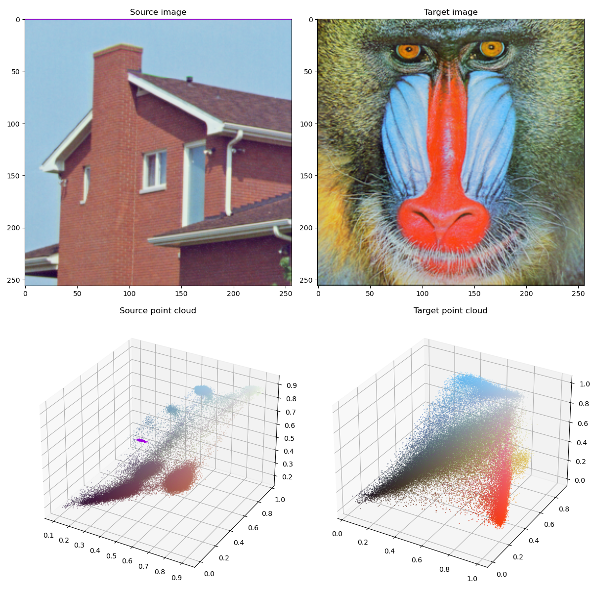
Our source and target samples are clouds of 3D points, each of whom encodes the RGB color of a pixel in a standard test image. We can then define a pair of discrete probability measures on our color space $[0,1{]}^3$:

$$\alpha =\frac{1}{N}\sum _{i=1}^N{\delta }_{x_i},\beta =\frac{1}{M}\sum _{j=1}^M{\delta }_{y_j}.$$

sampling = 8 if not use_cuda else 1

X_i = RGB_cloud("data/house_256.png", sampling, dtype)
Y_j = RGB_cloud("data/mandrill_256.png", sampling, dtype)

fig = plt.figure(figsize=(12, 12))
ax = fig.add_subplot(2, 2, 1)
display_image(ax, X_i)
ax.set_title("Source image")
ax = fig.add_subplot(2, 2, 2)
display_image(ax, Y_j)
ax.set_title("Target image")

ax = fig.add_subplot(2, 2, 3, projection="3d")
display_cloud(ax, X_i)
ax.set_title("Source point cloud")
ax = fig.add_subplot(2, 2, 4, projection="3d")
display_cloud(ax, Y_j)
ax.set_title("Target point cloud")
plt.tight_layout()

/home/code/geomloss/geomloss/examples/optimal_transport/plot_optimal_transport_color.py:38: DeprecationWarning: Starting with ImageIO v3 the behavior of this function will switch to that of iio.v3.imread. To keep the current behavior (and make this warning disappear) use `import imageio.v2 as imageio` or call `imageio.v2.imread` directly.
  img = imageio.imread(fname)  # RGB

Color transfer through gradient descent

To showcase the properties of the Sinkhorn divergence ${\text{S}}_{\epsilon ,\rho }$, we now follow the steps of the Optimal Transport example with custom parameters.

def color_transfer(loss, lr=1):
    """Flows along the gradient of the loss function.

    Parameters:
        loss ((x_i,y_j) -> torch float number):
            Real-valued loss function.
        lr (float, default = 1):
            Learning rate, i.e. time step.
    """

    # Parameters for the gradient descent
    Nsteps = 11
    display_its = [1, 10]

    # Make sure that we won't modify the reference samples
    x_i, y_j = X_i.clone(), Y_j.clone()

    # We're going to perform gradient descent on Loss(α, β)
    # wrt. the positions x_i of the diracs masses that make up α:
    x_i.requires_grad = True

    t_0 = time.time()

    plt.figure(figsize=(12, 12))
    k = 3
    ax = plt.subplot(2, 2, 1)
    display_image(ax, X_i)
    ax.set_title("Source image")
    plt.xticks([], [])
    plt.yticks([], [])
    ax = plt.subplot(2, 2, 2)
    display_image(ax, Y_j)
    ax.set_title("Target image")
    plt.xticks([], [])
    plt.yticks([], [])

    for i in range(Nsteps):  # Euler scheme ===============
        # Compute cost and gradient
        L_αβ = loss(x_i, y_j)
        [g] = torch.autograd.grad(L_αβ, [x_i])

        if i in display_its:  # display
            ax = plt.subplot(2, 2, k)
            display_image(ax, x_i)
            ax.set_title("it = {}".format(i))
            k = k + 1
            plt.xticks([], [])
            plt.yticks([], [])

        # in-place modification of the tensor's values
        x_i.data -= lr * len(x_i) * g

    plt.title(
        "it = {}, elapsed time: {:.2f}s/it".format(i, (time.time() - t_0) / Nsteps)
    )
    plt.tight_layout()

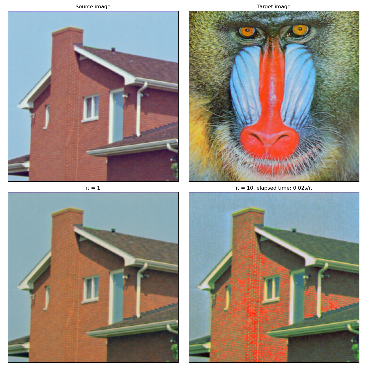
Wasserstein-2 Optimal Transport

When p = 2, the (normalized) Lagrangian gradient of the Sinkhorn divergence $v_i=\frac{1}{{\alpha }_i}{\mathrm{\nabla }}_{x_i}{\text{S}}_{\epsilon ,\rho }(\alpha ,\beta )$ defines a “Brenier map” whose smoothness and maximum reach can be tuned with the $\text{blur}=\sqrt{\epsilon }$ and $\text{reach}=\sqrt{\rho }$ parameters.

Crucially, when $(\epsilon ,\rho )\ne (0,+\mathrm{\infty })$, the overlap between the transported and target measures is not perfect. As we iterate our gradient descent on the colors $x_i\in {\mathbb{R}}^3$, we will thus transition from a smooth deformation of the source histogram to a precise deformation that overfits on the target color distribution.

color_transfer(SamplesLoss("sinkhorn", blur=0.3))

Clipping input data to the valid range for imshow with RGB data ([0..1] for floats or [0..255] for integers). Got range [-9.75281e-06..0.88715476].
Clipping input data to the valid range for imshow with RGB data ([0..1] for floats or [0..255] for integers). Got range [-0.023618542..1.2329485].

In most applications, the color transfer obtained after one, smooth update is more appropriate than the “perfect” matching, solution of the Monge problem. Fortunately, this smooth color transfer is also easier to compute!

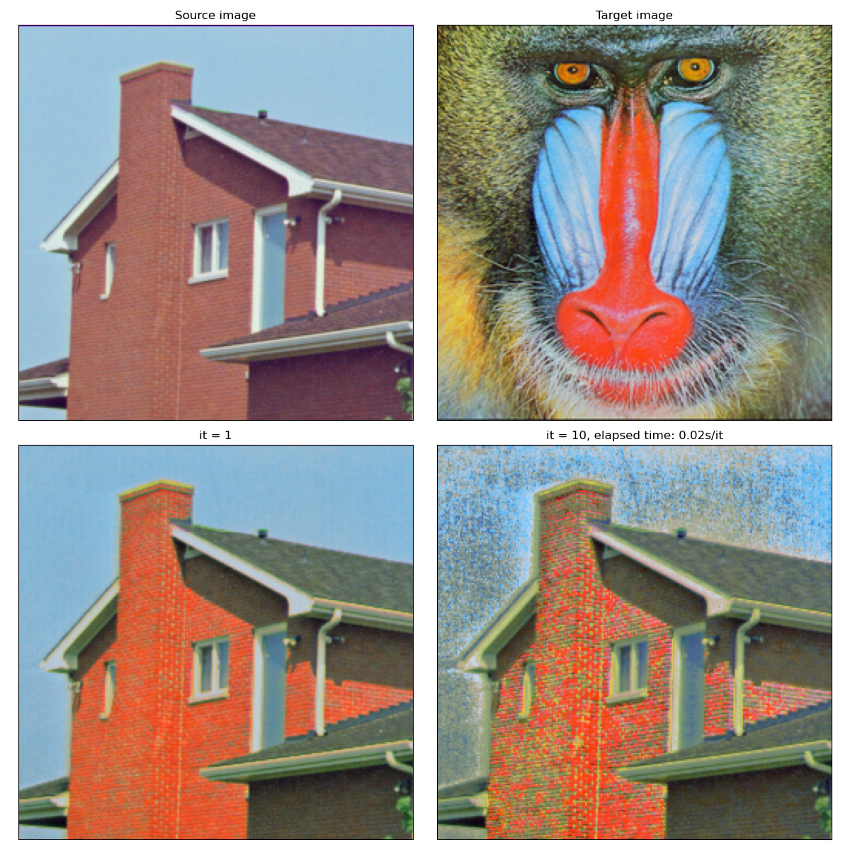
Feel free to play around with the input features (i.e. the coordinates system on the color space) and the blur parameter, which allows you to be more or less precise in the first few iterations:

color_transfer(SamplesLoss("sinkhorn", blur=0.1))

Clipping input data to the valid range for imshow with RGB data ([0..1] for floats or [0..255] for integers). Got range [0.012572595..1.0214131].
Clipping input data to the valid range for imshow with RGB data ([0..1] for floats or [0..255] for integers). Got range [-0.015074465..1.0201979].

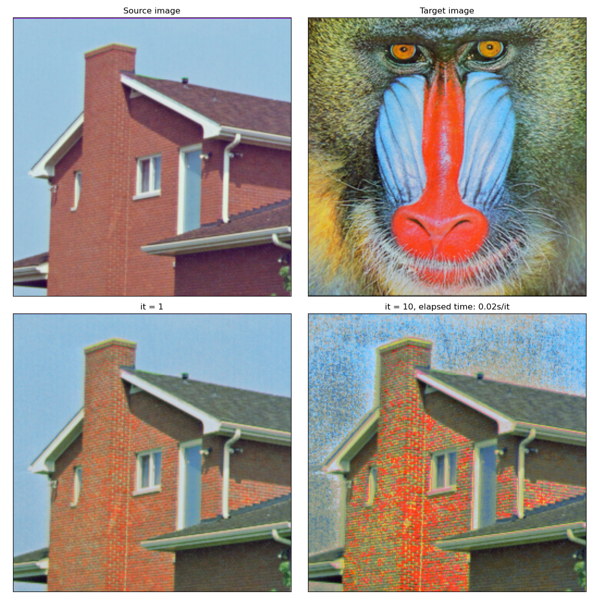
Going further, the reach parameter allows you to define a maximum transportation distance in the color space. In real-life applications, you may want to apply this simple algorithm on a higher-dimensional feature space (e.g. position + color), and thus get quasi-smooth matchings at a low computational cost.

color_transfer(SamplesLoss("sinkhorn", blur=0.1, reach=0.4))

plt.show()

Clipping input data to the valid range for imshow with RGB data ([0..1] for floats or [0..255] for integers). Got range [-0.017584927..1.0228894].