Wasserstein barycenters in 1D

Let’s compute Wasserstein barycenters with a Sinkhorn divergence, using Eulerian and Lagrangian optimization schemes.

Setup

import numpy as np
import matplotlib.pyplot as plt
from sklearn.neighbors import KernelDensity  # display as density curves

import torch
from geomloss import SamplesLoss

use_cuda = torch.cuda.is_available()
dtype = torch.cuda.FloatTensor if use_cuda else torch.FloatTensor

Dataset

Given a weight \(w\in[0,1]\) and two endpoint measures \(\alpha\) and \(\beta\), we wish to compute the Sinkhorn barycenter

\[\gamma^\star ~=~ \arg\min_{\gamma}~ (1-w)\cdot\text{S}_{\varepsilon,\rho}(\gamma,\alpha) \,+\, w\cdot\text{S}_{\varepsilon,\rho}(\gamma,\beta),\]

which coincides with \(\alpha\) when \(w=0\) and with \(\beta\) when \(w=1\).

If our input measures

\[\alpha ~=~ \frac{1}{M}\sum_{i=1}^M \delta_{x_i}, ~~~ \beta ~=~ \frac{1}{M}\sum_{j=1}^M \delta_{y_j},\]

are fixed, the optimization problem above is known to be convex with respect to the weights \(\gamma_k\) of the variable measure

\[\gamma ~=~ \sum_{k=1}^N \gamma_k\,\delta_{z_k}.\]

N, M = (50, 50) if not use_cuda else (500, 500)

t_i = torch.linspace(0, 1, M).type(dtype).view(-1, 1)
t_j = torch.linspace(0, 1, M).type(dtype).view(-1, 1)

X_i, Y_j = 0.1 * t_i, 0.2 * t_j + 0.8  # Intervals [0., 0.1] and [.8, 1.].

In this notebook, we thus propose to solve the barycentric optimization problem through a (quasi-)convex optimization on the (log-)weights \(\log(\gamma_k)\) - with fixed \(\delta_{z_k}\)’s - and through a well-conditioned descent on the samples’ positions \(\delta_{z_k}\) - with uniform weights \(\gamma_k = 1/N\).

In both sections (Eulerian vs. Lagrangian), we’ll start from a uniform sample on the unit interval:

t_k = torch.linspace(0, 1, N).type(dtype).view(-1, 1)
Z_k = t_k

Display routine

We display our samples using (smoothed) density curves, computed with a straightforward Gaussian convolution:

t_plot = np.linspace(-0.1, 1.1, 1000)[:, np.newaxis]


def display_samples(ax, x, color, weights=None, blur=0.002):
    """Displays samples on the unit interval using a density curve."""
    kde = KernelDensity(kernel="gaussian", bandwidth=blur).fit(
        x.data.cpu().numpy(),
        sample_weight=None if weights is None else weights.data.cpu().numpy(),
    )
    dens = np.exp(kde.score_samples(t_plot))
    dens[0] = 0
    dens[-1] = 0
    ax.fill(t_plot, dens, color=color)

Eulerian gradient flow

Taking advantage of the convexity of Sinkhorn divergences with respect to the measures’ weights, we first solve the barycentric optimization problem through a (quasi-convex) Eulerian descent on the log-weights \(l_k = \log(\gamma_k)\):

from geomloss.examples.optimal_transport.model_fitting import (
    fit_model,
)  # Wrapper around scipy.optimize
from torch.nn import Module, Parameter  # PyTorch syntax for optimization problems


class Barycenter(Module):
    """Abstract model for the computation of Sinkhorn barycenters."""

    def __init__(self, loss, w=0.5):
        super(Barycenter, self).__init__()
        self.loss = loss  # Sinkhorn divergence to optimize
        self.w = w  # Interpolation coefficient
        # We copy the reference starting points, to prevent in-place modification:
        self.x_i, self.y_j, self.z_k = X_i.clone(), Y_j.clone(), Z_k.clone()

    def fit(self, display=False, tol=1e-10):
        """Uses a custom wrapper around the scipy.optimize module."""
        fit_model(self, method="L-BFGS", lr=1.0, display=display, tol=tol, gtol=tol)

    def weights(self):
        """The default weights are uniform, equal to 1/N."""
        return (torch.ones(len(self.z_k)) / len(self.z_k)).type_as(self.z_k)

    def plot(self, nit=0, cost=0, ax=None, title=None):
        """Displays the descent using a custom 'waffle' layout.

        N.B.: As the L-BFGS descent typically induces high-frequencies in
              the optimization process, we blur the 'interpolating' measure
              a little bit more than the two endpoints.
        """
        if ax is None:
            if nit == 0 or nit % 16 == 4:
                plt.pause(0.01)
                plt.figure(figsize=(16, 4))

            if nit <= 4 or nit % 4 == 0:
                if nit < 4:
                    index = nit + 1
                else:
                    index = (nit // 4 - 1) % 4 + 1
                ax = plt.subplot(1, 4, index)

        if ax is not None:
            display_samples(ax, self.x_i, (0.95, 0.55, 0.55))
            display_samples(ax, self.y_j, (0.55, 0.55, 0.95))
            display_samples(
                ax, self.z_k, (0.55, 0.95, 0.55), weights=self.weights(), blur=0.005
            )

            if title is None:
                ax.set_title("nit = {}, cost = {:3.4f}".format(nit, cost))
            else:
                ax.set_title(title)

            ax.axis([-0.1, 1.1, -0.1, 20.5])
            ax.set_xticks([], [])
            ax.set_yticks([], [])
            plt.tight_layout()


class EulerianBarycenter(Barycenter):
    """Barycentric model with fixed locations z_k, as we optimize on the log-weights l_k."""

    def __init__(self, loss, w=0.5):
        super(EulerianBarycenter, self).__init__(loss, w)

        # We're going to work with variable weights, so we should explicitely
        # define the (uniform) weights on the "endpoint" samples:
        self.a_i = (torch.ones(len(self.x_i)) / len(self.x_i)).type_as(self.x_i)
        self.b_j = (torch.ones(len(self.y_j)) / len(self.y_j)).type_as(self.y_j)

        # Our parameter to optimize: the logarithms of our weights
        self.l_k = Parameter(torch.zeros(len(self.z_k)).type_as(self.z_k))

    def weights(self):
        """Turns the l_k's into the weights of a positive probabilty measure."""
        return torch.nn.functional.softmax(self.l_k, dim=0)

    def forward(self):
        """Returns the cost to minimize."""
        c_k = self.weights()
        return self.w * self.loss(c_k, self.z_k, self.a_i, self.x_i) + (
            1 - self.w
        ) * self.loss(c_k, self.z_k, self.b_j, self.y_j)

For this first experiment, we err on the side of caution and use a small blur value in conjuction with a large scaling coefficient - i.e. a large number of iterations in the Sinkhorn loop:

EulerianBarycenter(SamplesLoss("sinkhorn", blur=0.001, scaling=0.99)).fit(display=True)

• 
• 
• 
• 
• 
• 
• 
• 
• 
• 
• 

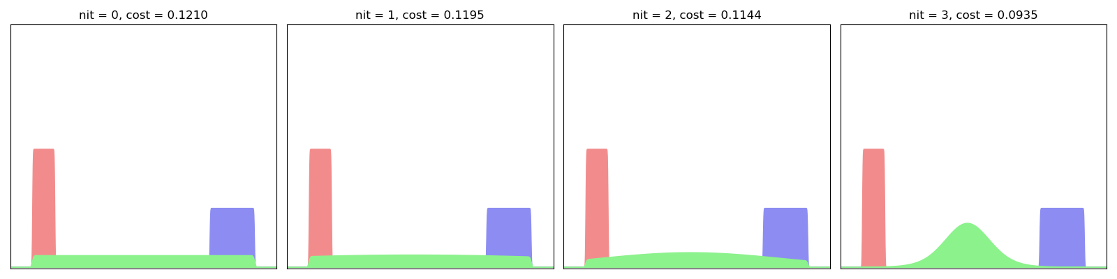
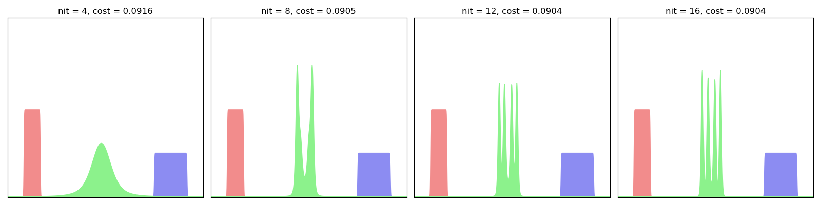
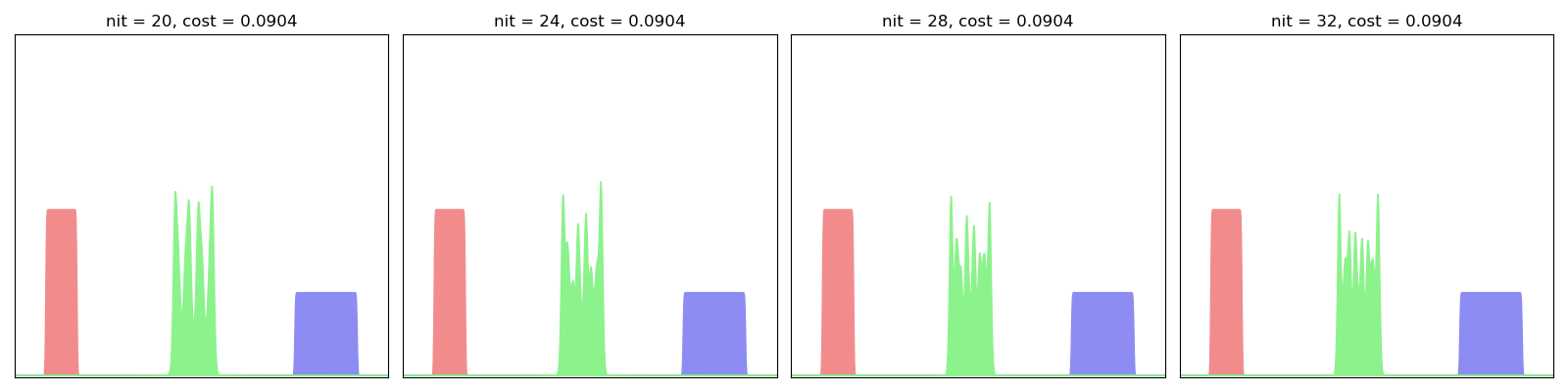
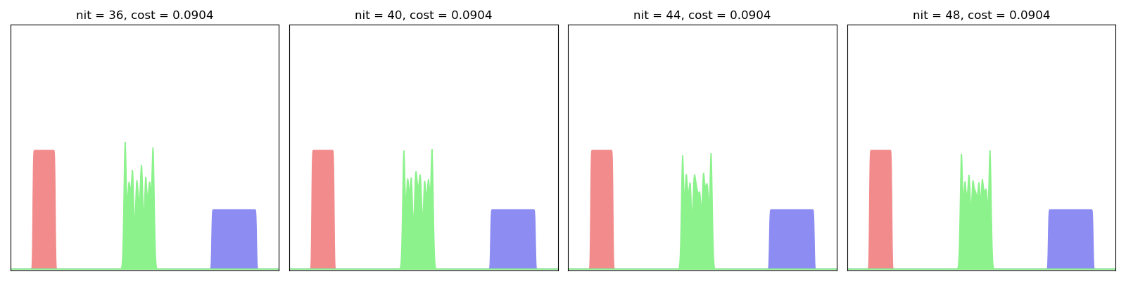
As evidenced here, the Eulerian descent fits one by one the Fourier modes of the “true” Wasserstein barycenter: we start from a Gaussian blob and progressively integrate the higher frequencies, slowly converging towards a sharp step function.

Lagrangian gradient flow

The procedure above is theoretically sound (thanks to the convexity of Sinkhorn divergences), but may be too slow for practical purposes. A simple workaround is to tackle the barycentric interpolation problem using a Lagrangian, particular scheme and optimize our weighted loss with respect to the samples’ positions:

class LagrangianBarycenter(Barycenter):
    def __init__(self, loss, w=0.5):
        super(LagrangianBarycenter, self).__init__(loss, w)

        # Our parameter to optimize: the locations of the input samples
        self.z_k = Parameter(Z_k.clone())

    def forward(self):
        """Returns the cost to minimize."""
        # By default, the weights are uniform and sum up to 1:
        return self.w * self.loss(self.z_k, self.x_i) + (1 - self.w) * self.loss(
            self.z_k, self.y_j
        )

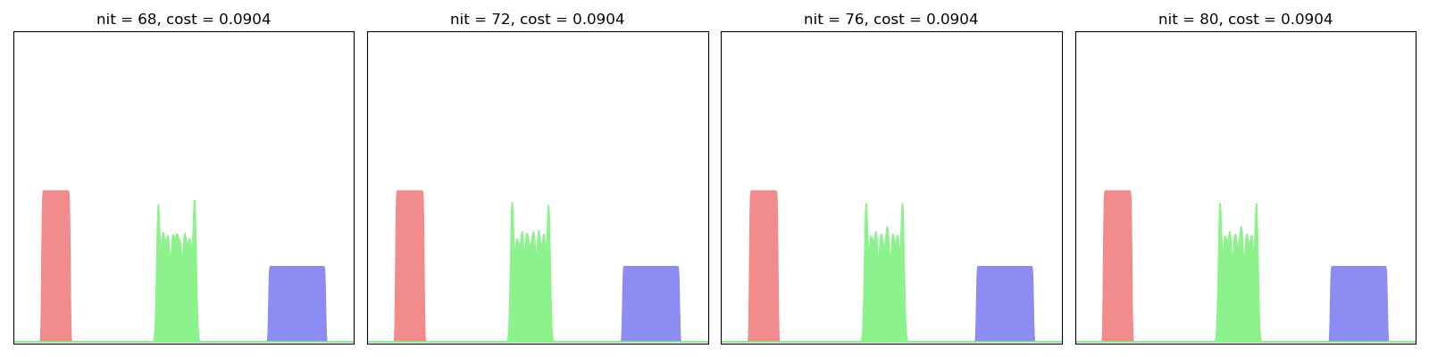
As evidenced below, this algorithm converges quickly towards a decent interpolator, even for small-ish values of the scaling coefficient:

LagrangianBarycenter(SamplesLoss("sinkhorn", blur=0.01, scaling=0.9)).fit(display=True)

• 
• 
• 

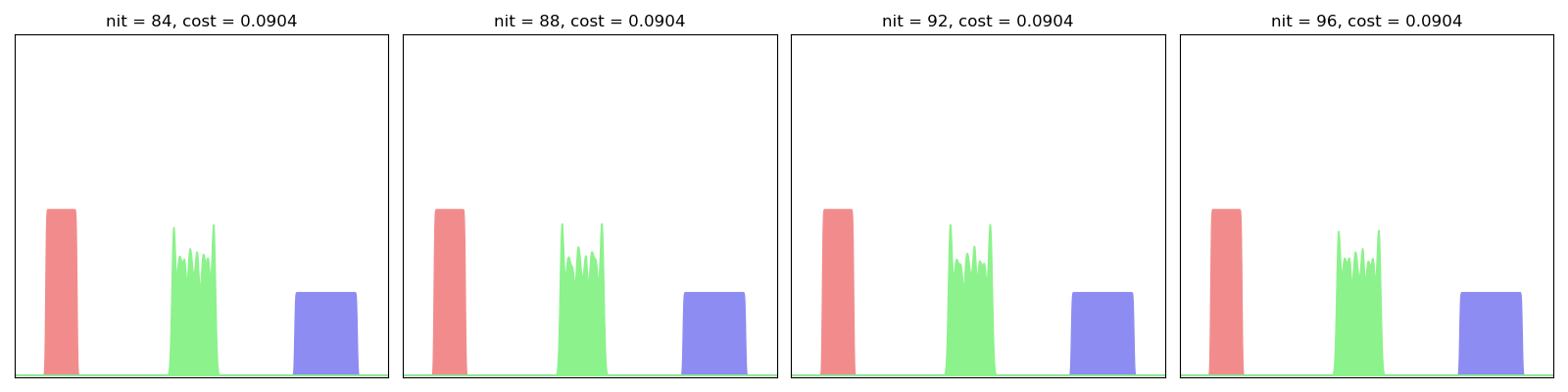
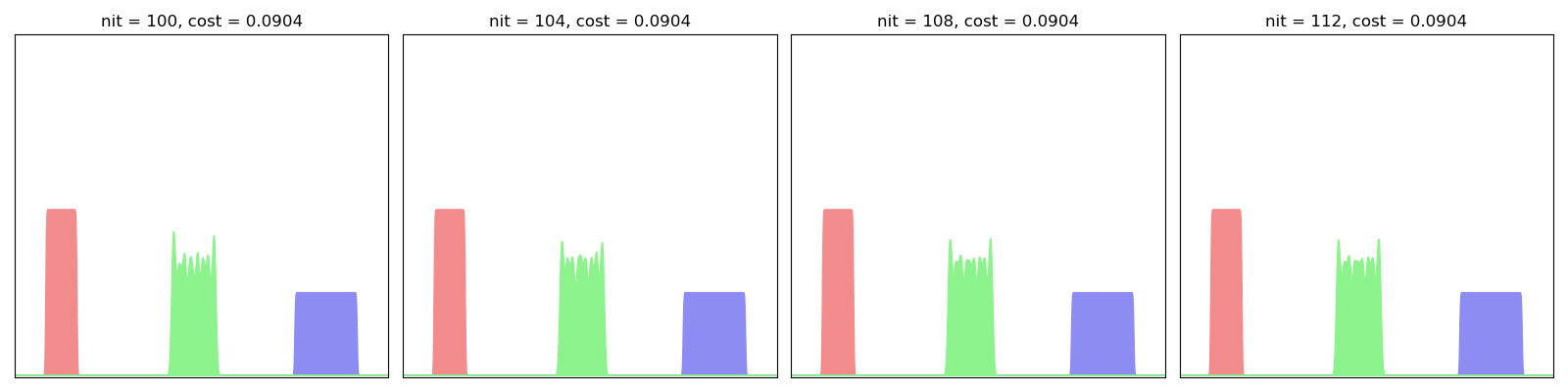
This algorithm can be understood as a generalization of Optimal Transport registration to multi-target applications and can be used to compute efficiently some Wasserstein barycenters in 2D. The trade-off between speed and accuracy (especially with respect to oscillating artifacts) can be tuned with the tol and scaling parameters:

LagrangianBarycenter(SamplesLoss("sinkhorn", blur=0.01, scaling=0.5)).fit(
    display=True, tol=1e-5
)
plt.show()