Wasserstein barycenters in 2D

Let’s compute pseudo-Wasserstein barycenters between 2D densities, using the gradient of the Sinkhorn divergence as a cheap approximation of the Monge map.

Setup

import numpy as np
import matplotlib.pyplot as plt
from imageio import imread
from sklearn.neighbors import KernelDensity
from torch.nn.functional import avg_pool2d

import torch
from geomloss import SamplesLoss

use_cuda = torch.cuda.is_available()
dtype = torch.cuda.FloatTensor if use_cuda else torch.FloatTensor

Dataset

In this tutorial, we work with square images understood as densities on the unit square.

def grid(W):
    x, y = torch.meshgrid([torch.arange(0.0, W).type(dtype) / W] * 2, indexing="xy")
    return torch.stack((x, y), dim=2).view(-1, 2)


def load_image(fname):
    img = np.mean(imread(fname), axis=2)  # Grayscale
    img = (img[:, :]) / 255.0
    return 1 - img  # black = 1, white = 0


def as_measure(fname, size):
    weights = torch.from_numpy(load_image(fname)).type(dtype)
    sampling = weights.shape[0] // size
    weights = (
        avg_pool2d(weights.unsqueeze(0).unsqueeze(0), sampling).squeeze(0).squeeze(0)
    )
    weights = weights / weights.sum()

    samples = grid(size)
    return weights.view(-1), samples

To perform Lagrangian computations, we turn these png bitmaps into weighted point clouds, regularly spaced on a grid:

N, M = (8, 8) if not use_cuda else (128, 64)

A, B = as_measure("data/A.png", M), as_measure("data/B.png", M)
C, D = as_measure("data/C.png", M), as_measure("data/D.png", M)

/home/code/geomloss/geomloss/examples/optimal_transport/plot_wasserstein_barycenters_2D.py:40: DeprecationWarning: Starting with ImageIO v3 the behavior of this function will switch to that of iio.v3.imread. To keep the current behavior (and make this warning disappear) use `import imageio.v2 as imageio` or call `imageio.v2.imread` directly.
  img = np.mean(imread(fname), axis=2)  # Grayscale

The starting point of our algorithm is a finely grained uniform sample on the unit square:

x_i = grid(N).view(-1, 2)
a_i = (torch.ones(N * N) / (N * N)).type_as(x_i)

x_i.requires_grad = True

Display routine

To display our interpolating point clouds, we put points into square bins and display the resulting density, using an appropriate threshold to mitigate quantization artifacts:

import matplotlib

matplotlib.rc("image", cmap="gray")

grid_plot = grid(M).view(-1, 2).cpu().numpy()


def display_samples(ax, x, weights=None):
    """Displays samples on the unit square using a simple binning algorithm."""
    x = x.clamp(0, 1 - 0.1 / M)
    bins = (x[:, 0] * M).floor() + M * (x[:, 1] * M).floor()
    count = bins.int().bincount(weights=weights, minlength=M * M)
    ax.imshow(
        count.detach().float().view(M, M).cpu().numpy(),
        vmin=0,
        vmax=0.5 * count.max().item(),
    )

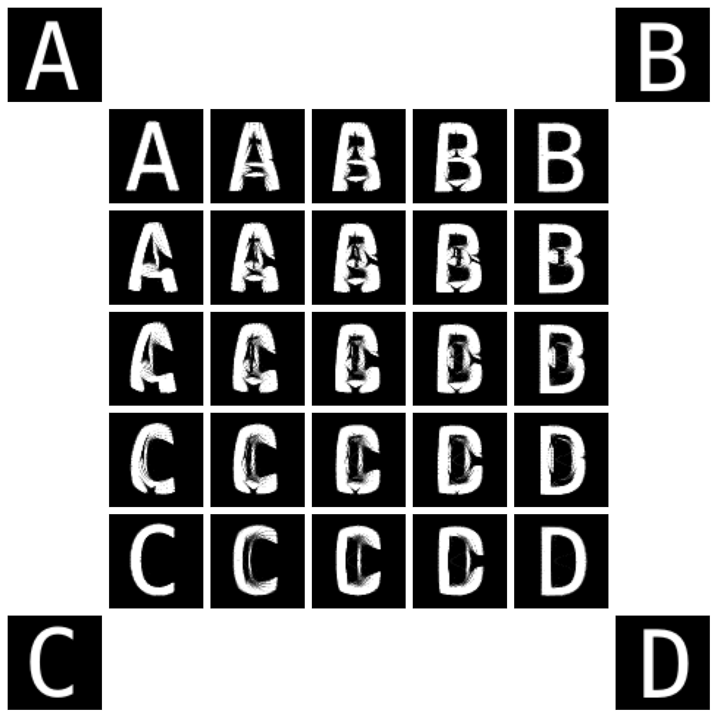
In the notebook on Wasserstein barycenters, we’ve seen how to solve generic optimization problems of the form

\[\begin{split}\alpha^\star~=~\arg\min_\alpha w_a \cdot \text{S}_{\varepsilon,\rho}(\,\alpha,\,A\,) ~&+~ w_b \cdot \text{S}_{\varepsilon,\rho}(\,\alpha,\,B\,) \\ ~+~ w_c \cdot \text{S}_{\varepsilon,\rho}(\,\alpha,\,C\,) ~&+~ w_d \cdot \text{S}_{\varepsilon,\rho}(\,\alpha,\,D\,)\end{split}\]

using Eulerian and Lagrangian schemes.

Focusing on the Lagrangian descent, a single (weighted) gradient step on the points \(x_i\) that make up the variable distribution \(\alpha = \sum_{i=1}^N \alpha_i \delta_{x_i}\) results in an update

\[x_i ~\gets~ x_i + w_a\cdot v_i^A + w_b\cdot v_i^B + w_c\cdot v_i^C + w_d\cdot v_i^D,\]

where the \(\,v_i^A\,=\,-\tfrac{1}{\alpha_i}\nabla_{x_i}\text{S}_{\varepsilon,\rho}(\,\alpha,\,A\,)\,\), etc. are the displacement vectors that map the starting (uniform) sample \(\alpha\) to the target measures \(A\), \(B\), \(C\) and \(D\).

Loss = SamplesLoss("sinkhorn", blur=0.01, scaling=0.9)
models = []
for (b_j, y_j) in [A, B, C, D]:
    L_ab = Loss(a_i, x_i, b_j, y_j)
    [g_i] = torch.autograd.grad(L_ab, [x_i])
    models.append(x_i - g_i / a_i.view(-1, 1))

a, b, c, d = models

If the weights \(w_k\) sum up to 1, this update is a barycentric combination of the target points \(x_i + v_i^A\), \(~\dots\,\), \(x_i + v_i^D\), images of the source sample \(x_i\) under the action of the generalized Monge/Brenier maps that transport our uniform sample onto the four target measures.

Using the resulting sample as an ersatz for the true Wasserstein barycenter is thus an approximation that holds in dimension 1, and is reasonable for most applications. As evidenced below, it allows us to interpolate between arbitrary densities at a low numerical cost:

plt.figure(figsize=(14, 14))

# Display the target measures in the corners of our Figure
ax = plt.subplot(7, 7, 1)
ax.imshow(A[0].reshape(M, M).cpu())
ax.set_xticks([], [])
ax.set_yticks([], [])
ax = plt.subplot(7, 7, 7)
ax.imshow(B[0].reshape(M, M).cpu())
ax.set_xticks([], [])
ax.set_yticks([], [])
ax = plt.subplot(7, 7, 43)
ax.imshow(C[0].reshape(M, M).cpu())
ax.set_xticks([], [])
ax.set_yticks([], [])
ax = plt.subplot(7, 7, 49)
ax.imshow(D[0].reshape(M, M).cpu())
ax.set_xticks([], [])
ax.set_yticks([], [])

# Display the interpolating densities as a 5x5 waffle plot
for i in range(5):
    for j in range(5):
        x, y = j / 4, i / 4
        barycenter = (
            (1 - x) * (1 - y) * a + x * (1 - y) * b + (1 - x) * y * c + x * y * d
        )

        ax = plt.subplot(7, 7, 7 * (i + 1) + j + 2)
        display_samples(ax, barycenter)
        ax.set_xticks([], [])
        ax.set_yticks([], [])

plt.tight_layout()
plt.show()