Label transfer with Optimal Transport

Let’s use a regularized Optimal Transport plan to transfer labels from one point cloud to another.

Setup

Standard imports:

import numpy as np
import matplotlib.pyplot as plt
import time
import torch

use_cuda = torch.cuda.is_available()
dtype = torch.cuda.FloatTensor if use_cuda else torch.FloatTensor

Display routines:

import imageio


def load_image(fname):
    img = imageio.imread(fname)[::-1, :, :3]  # RGB, without Alpha channel
    return img / 255.0  # Normalized to [0,1]


def display_samples(ax, x, color="black"):
    x_ = x.detach().cpu().numpy()
    if type(color) is not str:
        color = color.detach().cpu().numpy()
    ax.scatter(x_[:, 0], x_[:, 1], 25 * 500 / len(x_), color, edgecolors="none")

Draw labeled samples from an RGB image:

from random import choices


def draw_samples(fname, n, dtype=torch.FloatTensor, labels=False):
    A = load_image(fname)
    xg, yg = np.meshgrid(
        np.arange(A.shape[0]),
        np.arange(A.shape[1]),
        indexing="xy",
    )

    # Draw random coordinates according to the input density:
    A_gray = (1 - A).sum(2)
    grid = list(zip(xg.ravel(), yg.ravel()))
    dens = A_gray.ravel() / A_gray.sum()
    dots = np.array(choices(grid, dens, k=n))

    # Pick the correct labels:
    if labels:
        labs = A[dots[:, 1], dots[:, 0]].reshape((n, 3))

    # Normalize the coordinates to fit in the unit square, and add some noise
    dots = (dots.astype(float) + 0.5) / np.array([A.shape[0], A.shape[1]])
    dots += (0.5 / A.shape[0]) * np.random.standard_normal(dots.shape)

    if labels:
        return torch.from_numpy(dots).type(dtype), torch.from_numpy(labs).type(dtype)
    else:
        return torch.from_numpy(dots).type(dtype)

Dataset

Our source and target samples are drawn from measures whose densities are stored in simple PNG files. They allow us to define a pair of discrete probability measures:

\[\alpha ~=~ \frac{1}{N}\sum_{i=1}^N \delta_{x_i}, ~~~ \beta ~=~ \frac{1}{M}\sum_{j=1}^M \delta_{y_j},\]

with uniform weights \(\alpha_i = \tfrac{1}{N}\) and \(\beta_j = \tfrac{1}{M}\).

N, M = (500, 500) if not use_cuda else (10000, 10000)

X_i = draw_samples("data/threeblobs_a.png", N, dtype)
Y_j, l_j = draw_samples("data/threeblobs_b.png", M, dtype, labels=True)

/home/code/geomloss/geomloss/examples/optimal_transport/plot_optimal_transport_labels.py:31: DeprecationWarning: Starting with ImageIO v3 the behavior of this function will switch to that of iio.v3.imread. To keep the current behavior (and make this warning disappear) use `import imageio.v2 as imageio` or call `imageio.v2.imread` directly.
  img = imageio.imread(fname)[::-1, :, :3]  # RGB, without Alpha channel

In this tutorial, the \(y_j\)’s are endowed with color labels encoded as one-hot vectors \(\ell_j\) which are equal to:

• \((1,0,0)\) for red points,

• \((0,1,0)\) for green points,

• \((0,0,1)\) for blue points.

In the next few paragraphs, we’ll see how to use regularized Optimal Transport plans to transfer these labels from the \(y_j\)’s onto the \(x_i\)’s. But first, let’s display our source (noisy, labeled) and target point clouds:

plt.figure(figsize=(8, 8))
ax = plt.gca()
ax.scatter([10], [10])  # shameless hack to prevent a slight change of axis...

# Fancy display:
display_samples(ax, Y_j, l_j)
display_samples(ax, X_i)
ax.set_title("Source (Labeled) and Target  point clouds")

ax.axis([0, 1, 0, 1])
ax.set_aspect("equal", adjustable="box")
plt.tight_layout()

Regularized Optimal Transport

The SamplesLoss("sinkhorn") layer relies on a fast multiscale solver for the regularized Optimal Transport problem:

\[\begin{split}\text{OT}_\varepsilon(\alpha,\beta)~&=~ \min_{0 \leqslant \pi \ll \alpha\otimes\beta} ~\langle\text{C},\pi\rangle ~+~\varepsilon\,\text{KL}(\pi,\alpha\otimes\beta) \quad\text{s.t.}~~ \pi\,\mathbf{1} = \alpha ~~\text{and}~~ \pi^\intercal \mathbf{1} = \beta\\ &=~ \max_{f,g} ~~\langle \alpha,f\rangle + \langle \beta,g\rangle - \varepsilon\langle \alpha\otimes\beta, \exp \tfrac{1}{\varepsilon}[ f\oplus g - \text{C} ] - 1 \rangle,\end{split}\]

where \(\text{C}(x,y)=\tfrac{1}{p}\|x-y\|_2^p\) is a cost function on the feature space and \(\varepsilon\) is a positive regularization strength (the temperature) specified through the blur parameter \(\sigma = \varepsilon^{1/p}\). By default, SamplesLoss computes the unbiased (positive, definite) Sinkhorn divergence

\[\text{S}_\varepsilon(\alpha,\beta) ~=~ \text{OT}_\varepsilon(\alpha,\beta) - \tfrac{1}{2} \text{OT}_\varepsilon(\alpha,\alpha) - \tfrac{1}{2} \text{OT}_\varepsilon(\beta,\beta)\]

and returns a differentiable scalar value. But if we set the optional parameters debias to False and potentials to True, we will instead get access to the optimal dual potentials \(f\) and \(g\), solution of the \(\text{OT}_\varepsilon(\alpha,\beta)\) problem and respectively sampled on the \(x_i\)’s and \(y_j\)’s.

Note

By default, SamplesLoss("sinkhorn") uses an aggressive optimization heuristic where the blurring scale is halved between two successive iterations of the Sinkhorn loop, until reaching the required target value (scaling = .5). This choice is sensible when the Optimal Transport plan is used as a (cheap) gradient for an outer registration loop… But in this tutorial, setting the trade-off between speed (scaling \(\rightarrow\) 0) and accuracy (scaling \(\rightarrow\) 1) to a more conservative value of .9 is a sound decision.

from geomloss import SamplesLoss

blur = 0.05
OT_solver = SamplesLoss(
    "sinkhorn", p=2, blur=blur, scaling=0.9, debias=False, potentials=True
)
F_i, G_j = OT_solver(X_i, Y_j)

With a linear memory footprint, these two dual vectors encode a full transport plan on the product space \(\{x_i, i \in[1,N]\}\times\{y_j, j \in[1,M]\}\): the primal solution of the \(\text{OT}_\varepsilon(\alpha,\beta)\) problem is simply given through

\[\begin{split}\pi~&=~ \exp \tfrac{1}{\varepsilon}[f\oplus g - \text{C}] \cdot \alpha\otimes \beta \\ \text{i.e.}~~ \pi_{i,j}~&=~ \exp \tfrac{1}{\varepsilon}[f_i+ g_j - \text{C}(x_i,y_j)] \cdot \alpha_i \beta_j\end{split}\]

and is such that

\[\begin{split}\pi\,\mathbf{1}~=~\alpha, & \qquad \pi^\intercal\mathbf{1}~=~\beta \\ \text{i.e.}~~ \sum_{j=1}^M \pi_{i,j}~=~\alpha_i, &\qquad \sum_{i=1}^N \pi_{i,j}~=~\beta_j\end{split}\]

up to convergence in the Sinkhorn loop.

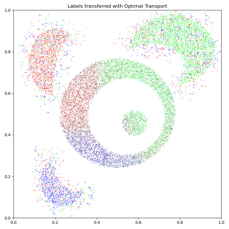
Transfer of labels. To transport our source labels \(\ell_j\) onto the \(x_i\)’s, a simple idea is to compute the barycentric combination

\[\text{Lab}_i ~=~ \frac{1}{\alpha_i} \sum_{j=1}^M \pi_{i,j} \ell_j ~\in~\mathbb{R}^3\]

for all points \(x_i\), interpreting the resulting vectors as soft assignments which may or may not be quantized back to discrete labels. Thanks to the fuzziness induced by the temperature \(\varepsilon = \text{blur}^p\) in the transport plan \(\pi_{i,j}\), the labelling noise is naturally smoothed out with labels \(\text{Lab}_i\) corresponding to averages over sets of source points whose diameters are roughly proportional to the blur scale.

Implicit computations. Keep in mind, however, that the full \(M\)-by-\(N\) matrix \(\pi\) may not fit in (GPU) memory if the number of samples \(\sqrt{M N}\) exceeds 10,000 or so. To break this memory bottleneck, we leverage the online map-reduce routines provided by the KeOps library which allow us to compute and sum the \(\pi_{i,j} \ell_j\)’s on-the-fly. We should simply come back to the expression of \(\pi_{i,j}\) and write:

\[\begin{split}\text{Lab}_i ~&=~ \sum_{j=1}^M \exp \tfrac{1}{\varepsilon}[f_i+ g_j - \text{C}(x_i,y_j)] \cdot \beta_j \ell_j \\ &=~ \frac{1}{M} \sum_{j=1}^M \exp \tfrac{1}{\varepsilon}[f_i+ g_j - \tfrac{1}{2}\|x_i-y_j\|^2] \cdot \ell_j.\end{split}\]

from pykeops.torch import generic_sum

# Define our KeOps CUDA kernel:
transfer = generic_sum(
    "Exp( (F_i + G_j - IntInv(2)*SqDist(X_i,Y_j)) / E ) * L_j",  # See the formula above
    "Lab = Vi(3)",  # Output:  one vector of size 3 per line
    "E   = Pm(1)",  # 1st arg: a scalar parameter, the temperature
    "X_i = Vi(2)",  # 2nd arg: one 2d-point per line
    "Y_j = Vj(2)",  # 3rd arg: one 2d-point per column
    "F_i = Vi(1)",  # 4th arg: one scalar value per line
    "G_j = Vj(1)",  # 5th arg: one scalar value per column
    "L_j = Vj(3)",
)  # 6th arg: one vector of size 3 per column

# And apply it on the data (KeOps is pretty picky on the input shapes...):
labels_i = (
    transfer(
        torch.Tensor([blur ** 2]).type(dtype),
        X_i,
        Y_j,
        F_i.view(-1, 1),
        G_j.view(-1, 1),
        l_j,
    )
    / M
)

That’s it! We may now display our target point cloud \((x_i)\) with its new set of labels:

# sphinx_gallery_thumbnail_number = 2
plt.figure(figsize=(8, 8))
ax = plt.gca()
ax.scatter([10], [10])  # shameless hack to prevent a slight change of axis...

# Fancy display:
display_samples(ax, Y_j, l_j)
display_samples(ax, X_i, labels_i.clamp(0, 1))
ax.set_title("Labels transferred with Optimal Transport")

ax.axis([0, 1, 0, 1])
ax.set_aspect("equal", adjustable="box")
plt.tight_layout()

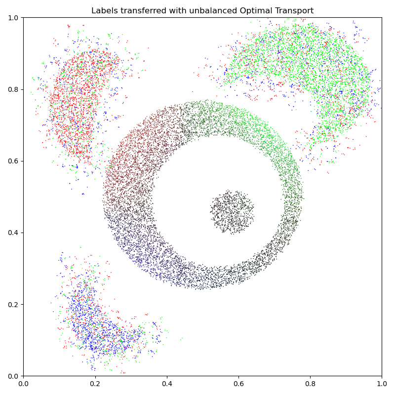
Unbalanced Optimal Transport

As evidenced above, the blur parameter allows us to smooth our optimal transport plan to remove noise in the final labelling. In most real-life situations, we may also wish to gain robustness against outliers by preventing samples from having too much influence outside of a fixed neighborhood.

SamplesLoss("sinkhorn") allows us to do so through the reach parameter, which is set to None (\(+\infty\)) by default and acts as a threshold on the maximal distance travelled by points in the assignment problem. From a theoretical point of view, this is done through the resolution of an unbalanced Optimal Transport problem:

\[\begin{split}\text{OT}_{\varepsilon,\rho}(\alpha,\beta)~&=~ \min_{0 \leqslant \pi \ll \alpha\otimes\beta} ~\langle\text{C},\pi\rangle ~+~\varepsilon\,\text{KL}(\pi,\alpha\otimes\beta) ~+~ \rho \, \text{KL}(\pi\,\mathbf{1},\alpha) ~+~ \rho \, \text{KL}(\pi^\intercal \mathbf{1},\beta) \\ &=~ \max_{f,g} ~~\rho\,\langle \alpha, 1 - e^{-f/\rho} \rangle ~+ \rho \,\langle \beta, 1 - e^{-g/\rho} \rangle \\ &\qquad\qquad~- \varepsilon\langle \alpha\otimes\beta, \exp \tfrac{1}{\varepsilon}[ f\oplus g - \text{C} ] - 1 \rangle,\end{split}\]

where the hard marginal constraints have been replaced by a soft Kullback-Leibler penalty whose strength is specified through a positive parameter \(\rho = \text{reach}^p\).

OT_solver = SamplesLoss(
    "sinkhorn", p=2, blur=blur, reach=0.2, scaling=0.9, debias=False, potentials=True
)
F_i, G_j = OT_solver(X_i, Y_j)

# And apply it on the data:
labels_i = (
    transfer(
        torch.Tensor([blur ** 2]).type(dtype),
        X_i,
        Y_j,
        F_i.view(-1, 1),
        G_j.view(-1, 1),
        l_j,
    )
    / M
)

As we display our new set of labels, we can check that colors don’t get transported beyond the specified reach = .2. Target points which are too far away from the source simply stay black, with a soft label \(\text{Lab}_i\) close to \((0,0,0)\):

plt.figure(figsize=(8, 8))
ax = plt.gca()
ax.scatter([10], [10])  # shameless hack to prevent a slight change of axis...

display_samples(ax, Y_j, l_j)
display_samples(ax, X_i, labels_i.clamp(0, 1))
ax.set_title("Labels transferred with unbalanced Optimal Transport")

ax.axis([0, 1, 0, 1])
ax.set_aspect("equal", adjustable="box")
plt.tight_layout()


plt.show()